Summary | Source files | Compilation | Precompiled | Gallery | References

Poincare

A program for the visualization of trajectories of Stokes parameters on the Poincaré sphere. The program generates MetaPost code as output.

Summary of the program

The Poincare computer program creates topographic maps of Stokes parameters [1], visualized as trajectories on the Poincare sphere [2]. The Poincare program generates MetaPost source code as output, to be compiled into PostScript or Encapsulated PostScript [3], using John Hobby's MetaPost compiler or anything that understands the MetaPost syntax. I have used the Poincare program extensively in my research career, and the program has been continuously updated for almost nine years by now, in fact the oldest program I keep active in my stock. This program was used in the generation of the image that made it to the front page of issue 4 of J. Opt. A: Pure Appl. Opt., Vol. 2 (July 2000).

Current revision

Revision 1.23, as of 24/01/2014. Copyright © Fredrik Jonsson 1997-2014, under GPL.

Source files

Compilation

Compile the source code 'poincare.c' using the enclosed Makefile, or simply by executing

gcc -O2 -g -Wall -pedantic -ansi ./poincare.c -o ./poincare -lm

Precompiled executables

Example gallery

Application example 1

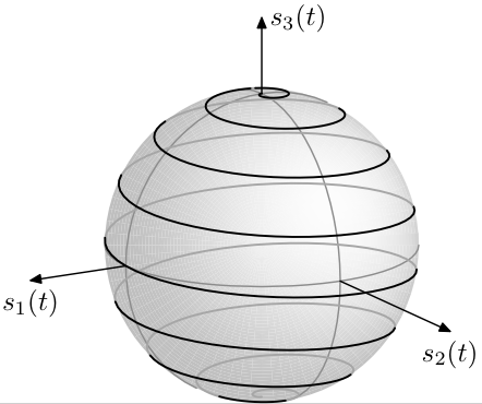
Figure 1. This is an example of a Poincare map of a spiraling helicoidal trajectory of Stokes parameters (artificially generated by an AWK script). The hidden parts of the trajectory is drawn as solid gray, and labels for the components of the Stokes vector (s₁(t),s₂(t),s₃(t)) are displayed at the corresponding axes.
[ Download MetaPost code | view source | Encapsulated PostScript image (689 kB) ]

Extract of Makefile for the generation of Fig. 1:

#
# example-a:
#
#    This is simply an example of a Poincare map of a spiraling
#    helicoidal trajectory of Stokes parameters. The hidden parts
#    of the trajectory is drawn as solid gray, and labels for the
#    components of the Stokes vector (s_1(t),s_2(t),s_3(t)) are
#    displayed at the corresponding axes.
#
example-a:
   make poincare
   @echo 1|$(AWK) 'BEGIN {n=440; pi=3.1415926535;}{\
   printf("p\n");\
   for (k=0;k<=n;k++) {\
      t=k/n; phi=t*16*pi; theta=t*pi;\
      x=cos(phi)*sin(theta); \
      y=sin(phi)*sin(theta); \
      z=cos(theta);\
      printf("%-6.4f %-6.4f %-6.4f\n",x,y,z);\
   }\
   printf("q\n");\
   }END{}' > example-a.dat
   @./poincare --verbose --normalize \
      --inputfile example-a.dat  --outputfile example-a.mp \
      --axislengths 0.3 1.7 0.3 2.4 0.3 1.5 \
      --axislabels  "s_1(t)" bot "s_2(t)" bot "s_3(t)" rt \
      --rotatephi 15.3  --rotatepsi -60.0 --shading 0.75 0.99 \
      --rhodivisor 50  --phidivisor 80  --scalefactor 20.0 \
      --paththickness 0.8 --arrowthickness 0.4
   @$(METAPOST) example-a.mp
   @$(TEX) -jobname=example-a '\input epsf\nopagenumbers\
      \centerline{\epsfxsize=155mm\epsfbox{example-a.1}}\bye'
   @$(DVIPS) $(DVIPSOPTS) example-a -o example-a.eps

---

Application example 2

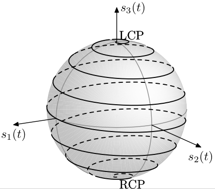
Figure 2. This example is similar to the one in the previous figure, but now with labels added at the beginning and end points of the trajectory (LCP and RCP, indicating the poles of left and right circular polarization states, respctivelty). These labels are added with the '--axislabels' option in the listed block of the Makefile. In addition, the appearance of hidden parts of the trajectory has been changed to dashed black, using the '--draw_hidden_dashed' option.
[ Download MetaPost code | view source | Encapsulated PostScript image (693 kB) ]

Extract of Makefile for the generation of Fig. 2:

# example-b:
#
#    This example figure is similar to example-a, but with labels
#    added to the beginning and end points of the trajectory (LCP
#    and RCP, respectively). In addition, the appearance of hidden
#    parts of the trajectory has been changed to dashed black.
#
example-b:
   make poincare
   @echo 1|$(AWK) 'BEGIN {n=440; pi=3.1415926535;}{\
   printf("p b urgt \"LCP\"\n");\
   for (k=0;k<=n;k++) {\
      t=k/n; phi=t*16*pi; theta=t*pi;\
      x=cos(phi)*sin(theta); \
      y=sin(phi)*sin(theta); \
      z=cos(theta);\
      printf("%-6.4f %-6.4f %-6.4f\n",x,y,z);\
   }\
   printf("q e lrgt \"RCP\"\n");\
   }END{}' > example-b.dat
   @./poincare --verbose --normalize --draw_hidden_dashed \
      --inputfile example-b.dat  --outputfile example-b.mp \
      --axislengths 0.3 1.7 0.3 2.4 0.3 1.5 \
      --axislabels  "s_1(t)" bot "s_2(t)" bot "s_3(t)" rt \
      --rotatephi 15.0 --rotatepsi -60.0 --shading 0.75 0.99 \
      --rhodivisor 50  --phidivisor 80  --scalefactor 20.0 \
      --paththickness 0.8 --arrowthickness 0.4
   @$(METAPOST) example-b.mp
   @$(TEX) -jobname=example-b '\input epsf\nopagenumbers\
      \centerline{\epsfxsize=155mm\epsfbox{example-b.1}}\bye'
   @$(DVIPS) $(DVIPSOPTS) example-b -o example-b.eps

---

Application example 3

In this example, several trajectories are mapped onto the same sphere. This is something useful for illustrating, for example, wave propagation in isotropic media, in which case the form of the Stokes trajectory is invariant under rotation around the s₃-axis of the coordinate system (s₁,s₂,s₃).

Extract of Makefile for the generation of the data files for Figs. 3:

example-c:
   make example-c-data-solid
   make example-c-data-chopped
   make example-c-solid
   make example-c-chopped
   make example-c-chopped-reversed
   make example-c-chopped-dash

example-c-data-solid:
   make poincare
   echo 1|$(AWK) 'BEGIN {jj=10; kk=90; pi=3.1415926535; \
      ta=0.1; tb=0.9;}{\
   for (j=1;j<=jj;j++) {\
      phia=(j/jj)*2*pi;\
      printf("p\n");\
      for (k=1;k<=kk;k++) {\
         t=ta+(k/kk)*(tb-ta); \
         phi=phia+t*1.2*pi; \
         theta=t*pi;\
         x=cos(phi)*sin(theta); \
         y=sin(phi)*sin(theta); \
         z=-cos(theta);\
         printf("%-6.4f %-6.4f %-6.4f\n",x,y,z);\
      }\
      printf("q\n");\
   }\
   }END{}' > example-cs.dat

example-c-data-chopped:
   make poincare
   @echo 1|$(AWK) 'BEGIN {jj=10; kk=90; mm=4; pi=3.1415926535; \
      ta=0.1; tb=0.9;}{\
   for (j=1;j<=jj;j++) {\
      phia=(j/jj)*2*pi;\
      dkk=kk/mm;\
      for (m=1;m<=mm;m++) {\
      printf("p\n");\
      for (k=1+(m-1)*dkk;k<=1+m*dkk;k++) {\
         t=ta+(k/kk)*(tb-ta); \
         phi=phia+t*1.2*pi; \
         theta=t*pi;\
         x=cos(phi)*sin(theta); \
         y=sin(phi)*sin(theta); \
         z=-cos(theta);\
         printf("%-6.4f %-6.4f %-6.4f\n",x,y,z);\
      }\
      printf("q\n");\
      }\
   }\
   }END{}' > example-cc.dat

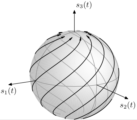
Figure 3(a). Multiple paths of trajectories mapped on the same sphere. In the basic configuration, each path will be draw by a single arrow indicating the directionality in traversing each path of the Stokes vector.
[ Download MetaPost code | view source | Encapsulated PostScript image (738 kB) ]

Extract of Makefile for the generation of Fig. 3(a):

example-c-solid:
   @./poincare --verbose --normalize --bezier \
      --inputfile example-cs.dat  --outputfile example-cs.mp \
      --axislengths 0.3 1.7 0.3 2.4 0.3 1.5 \
      --axislabels  "s_1(t)" bot "s_2(t)" bot "s_3(t)" urt \
      --rotatephi 15.0  --rotatepsi -60.0 --shading 0.75 0.99 \
      --rhodivisor 50  --phidivisor 80  --scalefactor 20.0 \
      --paththickness 0.8 --arrowthickness 0.4 \
      --arrowheadangle 20.0 --draw_paths_as_arrows
   $(METAPOST) example-cs.mp
   $(TEX) -jobname=example-cs '\input epsf\nopagenumbers\
      \centerline{\epsfxsize=155mm\epsfbox{example-cs.1}}\bye'
   $(DVIPS) $(DVIPSOPTS) example-cs -o example-cs.eps

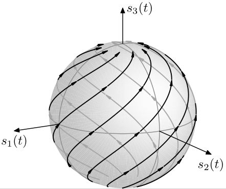
Figure 3(b). Same map as in previous figure, but now with the path arrows chopped up into several segments.
[ Download MetaPost code | view source | Encapsulated PostScript image (755 kB) ]

Extract of Makefile for the generation of Fig. 3(b):

example-c-chopped:
   @./poincare --verbose --normalize --bezier \
      --inputfile example-cc.dat  --outputfile example-cc.mp \
      --axislengths 0.3 1.7 0.3 2.4 0.3 1.5 \
      --axislabels  "s_1(t)" bot "s_2(t)" bot "s_3(t)" rt \
      --rotatephi 15.0  --rotatepsi -60.0 --shading 0.75 0.99 \
      --rhodivisor 50  --phidivisor 80  --scalefactor 20.0 \
      --paththickness 0.8 --arrowthickness 0.4 \
      --arrowheadangle 20.0 --draw_paths_as_arrows
   $(METAPOST) example-cc.mp
   $(TEX) -jobname=example-cc '\input epsf\nopagenumbers\
      \centerline{\epsfxsize=155mm\epsfbox{example-cc.1}}\bye'
   $(DVIPS) $(DVIPSOPTS) example-cc -o example-cc.eps

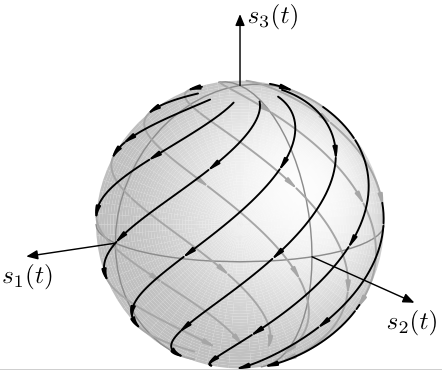
Figure 3(c). Same as previous figure, but now with the arrows reversed, using the '--reverse_arrow_paths' option.
[ Download MetaPost code | view source | Encapsulated PostScript image (773 kB) ]

Extract of Makefile for the generation of Fig. 3(c):

example-c-chopped-reversed:
   @./poincare --verbose --normalize --bezier \
      --inputfile example-cc.dat  --outputfile example-ccr.mp \
      --axislengths 0.3 1.7 0.3 2.4 0.3 1.5 \
      --axislabels  "s_1(t)" bot "s_2(t)" bot "s_3(t)" rt \
      --rotatephi 15.0  --rotatepsi -60.0 --shading 0.75 0.99 \
      --rhodivisor 50  --phidivisor 80  --scalefactor 20.0 \
      --paththickness 0.8 --arrowthickness 0.4 \
      --arrowheadangle 20.0 --draw_paths_as_arrows \
      --reverse_arrow_paths
   $(METAPOST) example-ccr.mp
   $(TEX) -jobname=example-ccr '\input epsf\nopagenumbers\
      \centerline{\epsfxsize=155mm\epsfbox{example-ccr.1}}\bye'
   $(DVIPS) $(DVIPSOPTS) example-ccr -o example-ccr.eps

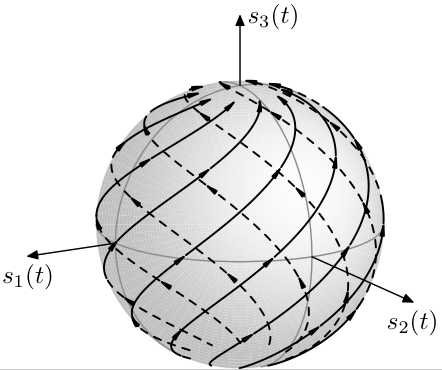
Figure 3(d).The effect of using the '--draw_hidden_dashed' option.
[ Download MetaPost code | view source | Encapsulated PostScript image (756 kB) ]

Extract of Makefile for the generation of Fig. 3(d):

example-c-chopped-dash:
   @./poincare --verbose --normalize --bezier --draw_hidden_dashed \
      --inputfile example-cc.dat  --outputfile example-cd.mp \
      --axislengths 0.3 1.7 0.3 2.4 0.3 1.5 \
      --axislabels  "s_1(t)" bot "s_2(t)" bot "s_3(t)" rt \
      --rotatephi 15.0  --rotatepsi -60.0 --shading 0.75 0.99 \
      --rhodivisor 50  --phidivisor 80  --scalefactor 20.0 \
      --paththickness 0.8 --arrowthickness 0.4 \
      --arrowheadangle 20.0 --draw_paths_as_arrows
   $(METAPOST) example-cd.mp
   $(TEX) -jobname=example-cd '\input epsf\nopagenumbers\
      \centerline{\epsfxsize=155mm\epsfbox{example-cd.1}}\bye'
   $(DVIPS) $(DVIPSOPTS) example-cd -o example-cd.eps

---

Application example 4

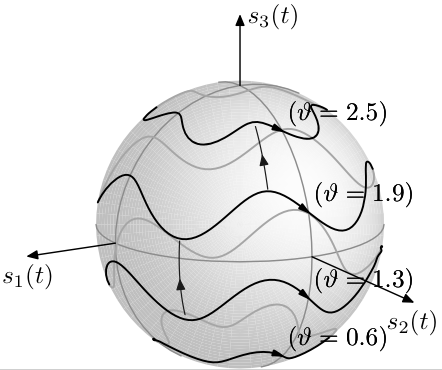
Figure 4. This example illustrates a set of closed trajectories, each being constructed out of concatenated pieces so as to create a plurality of arrow heads in each cycle. This example also illustrates how additional indicatory arrows may be included in the map by using the '--arrow' option repeatedly.
[ Download MetaPost code | view source | Encapsulated PostScript image (713 kB) ]

Extract of Makefile for the generation of Fig. 4:

#
# example-d:
#
#    This example illustrates a set of closed trajectories, each
#    being constructed out of concatenated pieces so as to create
#    a plurality of arrow heads in each cycle. This example also
#    illustrates how additional indicatory arrows may be included
#    in the map by using the '--arrow' option repeatedly.
#
example-d:
   make example-d-data
   make example-d-solid

example-d-data:
   make poincare
   echo 1|$(AWK) 'BEGIN {jj=5; kk=90; pi=3.1415926535; \
      ta=0.0; tb=1.0;}{\
   for (j=1;j<jj;j++) {\
      phia=(j/jj)*pi;\
      printf("p b urgt \"$$\(\\vartheta=%1.1f\)$$\"\n",phia);\
      for (k=0;k<=kk;k++) {\
         t=ta+(k/kk)*(tb-ta);\
         phi=t*2*pi+pi/2; \
         theta=(j/jj)*pi+(pi/17)*sin(phia)*cos(5*phi);\
         x=cos(phi)*sin(theta); \
         y=sin(phi)*sin(theta); \
         z=-cos(theta);\
         printf("%-6.4f %-6.4f %-6.4f\n",x,y,z);\
      }\
      printf("q\n");\
   }\
   }END{}' > example-d.dat

example-d-solid:
   @./poincare --verbose --normalize --bezier \
      --inputfile example-d.dat  --outputfile example-d.mp \
      --axislengths 0.3 1.7 0.3 2.4 0.3 1.5 \
      --axislabels  "s_1(t)" bot "s_2(t)" bot "s_3(t)" rt \
      --rotatephi 15.0  --rotatepsi -60.0 --shading 0.75 0.99 \
      --rhodivisor 50  --phidivisor 80  --scalefactor 20.0 \
      --paththickness 0.8 --arrowthickness 0.4 \
      --arrowheadangle 30.0 --draw_paths_as_arrows \
      --arrow 1.0 0.7 -0.58 1.0 0.7 0.15 0 0.9 \
      --arrow 0.28 0.9 0.52 0.3 0.9 1.5 0 0.9
   $(METAPOST) example-d.mp
   $(TEX) -jobname=example-d '\input epsf\nopagenumbers\
      \centerline{\epsfxsize=155mm\epsfbox{example-d.1}}\bye'
   $(DVIPS) $(DVIPSOPTS) example-d -o example-d.eps

---

Application example 5

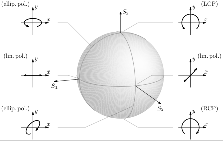
Figure 5. The following example of an application of the poincare program is taken from my PhD thesis, and illustrates how to append MetaPost code to the generated Poincare map, in this case an illustration of the interpretation of various parts of the Poincare sphere in terms of the polarization states, illustrated as the paths the point of the electrical field vector describes as one looks into the oncoming wave.

In this particular example, the MetaPost code in the file 'polstate.mp' contains all illustrations of the polarization state interpretation, and is appended via the 'input polstate.mp;' statement in the end of the generated file 'stoke.mp' (by using the '--auxsource' option when invoking the poincare program from the command line), which serves as a master source file when compiling the figure.
[ Download MetaPost code | view source | Encapsulated PostScript image (694 kB) ]

Extract of Makefile for the generation of Fig. 5:

example-stoke:
   make poincare
   @./poincare --verbose --normalize \
      --axislengths 0.3 1.6 0.3 2.7 0.3 1.5 \
      --axislabels  "S_1" bot "S_2" bot "S_3" rt \
      --rotatephi 15.0  --rotatepsi -70.0 \
      --shading 0.75 0.99 \
      --rhodivisor 50  --phidivisor 80  --scalefactor 25.0 \
      --outputfile stoke.mp --auxsource polstate.mp
   $(METAPOST) stoke.mp
   $(TEX) -jobname=stoke '\input epsf\nopagenumbers\
      \centerline{\epsfxsize=155mm\epsfbox{stoke.1}}\bye'
   $(DVIPS) $(DVIPSOPTS) stoke -o stoke.eps

References

[1] J. D. Jackson, Classical Electrodynamics, 2nd Edn. (Wiley, New York, 1975).

[2] The Poincaré sphere is classically denoted so after the French mathematician Henri Poincaré who in 1892 introduced it in his Théorie Mathématique de la Lumière, Vol. 2, Chapter 12, Pages 275-306 (Gauthiers-Villars, Paris, 1892).

[3] For information on the PostScript programming language, see for example the PostScript area on the website of Adobe Systems Inc., at http://www.adobe.com/products/postscript/ or the reference book "PostScript Language - Tutorial and Cookbook" (Adison-Wesley, Reading, Massachusetts, 1985), ISBN 0-201-10179-3.

Return to previous page

Leave a message

Your name:

Your email: (required)

Message:

Generated by ::emailform::