Lectures on Nonlinear Optics - Lecture 9
Two case studies in nonlinear optics
lect9.pdf [292 kB] Lecture 9 in Portable Document Format.
Contents
- General process for solving problems in nonlinear optics
- Formulation of the two case studies in this lecture
- Second harmonic generation
- Optical Kerr-effect - Field corrected refractive index
- References
In this lecture, we will focus on examples of electromagnetic wave propagation in nonlinear optical media, by applying the forms of Maxwell's equations as obtained in the eighth lecture to a set of particular nonlinear interactions as described by the previously formulated nonlinear susceptibility formalism.
The outline for this lecture is:
- General process for solving problems in nonlinear optics
- Second harmonic generation (SHG)
- Optical Kerr-effect
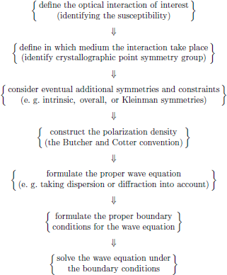
1. General process for solving problems in nonlinear optics
The typical steps in the process of solving a theoretical problem in nonlinear optics typically involve:
2. Formulation of the two case studies in this lecture
In order to illustrate the scheme as previously outlined, the following exercises serve as to give the connection between the susceptibilities, as extensively analysed from a quantum-mechanical basis in earlier lectures of this course, and the wave equation, derived from Maxwell's equations of motion for electromagnetic fields.
2.1. Case study I: Second harmonic generation in negative uniaxial media
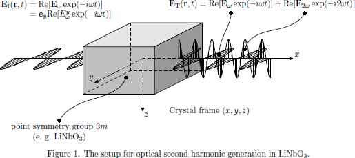
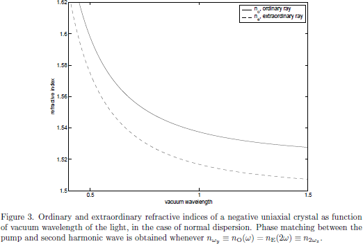
Consider a continuous pump wave at angular frequency ω, initially polarized in the y-direction and propagating in the positive x-direction of a negative uniaxial crystal of crystallographic point symmetry group 3m. (Examples of common crystals belonging to this class: β-BaB2O4 (beta barium borate, or BBO), LiNbO3 (lithium niobate).)
Task I (a): Formulate the polarization density of the medium for the pump and second harmonic wave.
Task I (b): Formulate the system of equations of motion for the electromagnetic fields.
Task I (c): Assuming no second harmonic signal present at the input, solve the equations of motion for the second harmonic field, using the non-depleted pump approximation, and derive an expression for the conversion efficiency of the second harmonic generation.
2.2. Case study II: Optical Kerr-effect - continuous wave case
In this setup, a monochromatic optical wave is propagating in the positive z-direction of an isotropic optical Kerr-medium. We here consider the case of a continuous optical wave, that is to say a non-pulsed beam. As will be shown in the Lecture 9, sufficiently intense optical pulses will in media possessing optical Kerr-effect experience different changes of the experienced refractive index at leading and trailing edges of the pulses, leading to the interesting phenomenon of optical solitons. However, basics first.
Task II (a): Formulate the polarization density of the medium for a wave polarized in the xy-plane.
Task II (b): Formulate the polarization density of the medium for a wave polarized in the x-direction.
Task II (c): Formulate the wave equation for continuous wave propagation in optical Kerr-media. The continuous wave is x-polarized and propagates in the positive z-direction.
Task II (d): For lossless media, solve the wave equation and give an expression for the nonlinear, intensity-dependent refractive index n = n0+n2|Eω|2.
3. Second harmonic generation
3.1. The optical interaction
In the case of second harmonic generation (SHG), two photons at angular frequency ω combine to a photon at twice the angular frequency,

This interaction is for the second harmonic wave (at angular frequency ω)described by the second order susceptibility

where, in the usual convention of Butcher and Cotter (as throughout applied this series of lectures), ωσ = 2ω is the generated second harmonic frequency of the light.
3.2. Symmetries of the medium
In this example we consider second harmonic generation in trigonal media of crystallographic point symmetry group 3m. (Example: LiNbO3, lithium niobate)
For this point symmetry group, the nonzero tensor elements of the first order susceptibility are (for example according to Table A3.1 in The Elements of Nonlinear Optics)
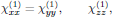
which gives the ordinary refractive indices
![$$
n_x(\omega)=n_y(\omega)=[1+\chi^{(1)}_{xx}(-\omega;\omega)]^{1/2}
\equiv n_{\rm O}(\omega)
$$](/research/lectures/lect9/web/images_80proc/lect9_eq_disp_004.png)
for waves components polarized in the $x$- or $y$-directions, and the extraordinary refractive index
![$$
n_z(\omega)=[1+\chi^{(1)}_{zz}(-\omega;\omega)]^{1/2}
\equiv n_{\rm E}(\omega)
$$](/research/lectures/lect9/web/images_80proc/lect9_eq_disp_005.png)
for the wave component polarized in the $z$-direction. Since we here are considering a negatively uniaxial crystal (see Butcher and Cotter, page 214), these refractive indices satisfy the inequality

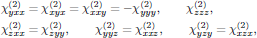
The nonzero tensor elements of the second order susceptibility are (for example according to Table A3.2 in {\sl The Elements of Nonlinear Optics})
 (1)
(1)3.3. Additional symmetries
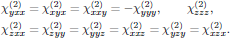
Intrinsic permutation symmetry for the case of second harmonic generation gives

which reduces the second order susceptibility in Eq. (1) to a set of 11 tensor elements, of which only 4 are independent. (We recall that the intrinsic permutation symmetry is always applicable, as being a consequence of the symmetrization described in lectures two and five.) Whenever Kleinman symmetry holds, the susceptibility is in addition symmetric under any permutation of the indices, which hence gives the additional relation

that is to say, reducing the second order susceptibility to a set of 11 tensor elements, of which only 3 are independent.
To summarize, the set of nonzero tensor elements describing second harmonic generation under Kleinman symmetry is
 (2)
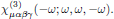
(2)For the pump field at angular frequency ω, the relevant susceptibility describing the interaction with the second harmonic wave is [1]
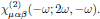
For an arbitrary frequency argument, this is the proper form of the susceptibility to use for the fundamental field, and this form generally differ from that of the susceptibilities for the second harmonic field. However, whenever Kleinman symmetry holds, the susceptibility for the fundamental field can be cast into the same parameters as for the second harmonic field, since
![$$
\eqalign{
\chi^{(2)}_{\mu\alpha\beta}(-\omega;2\omega,-\omega)
&=\big\{{\rm Apply\ overall\ permutation\ symmetry}\big\}\cr
&=\chi^{(2)}_{\alpha\mu\beta}(2\omega;-\omega,-\omega)\cr
&=\big\{{\rm Apply\ Kleinman\ symmetry}\big\}\cr
&=\chi^{(2)}_{\mu\alpha\beta}(2\omega;-\omega,-\omega)\cr
&=\big\{{\rm Apply\ reality\ condition\ [B.\,\&C.\,Eq.\,(2.43)]}\big\}\cr
&=[\chi^{(2)}_{\mu\alpha\beta}(-2\omega;\omega,\omega)]^*\cr
&=\chi^{(2)}_{\mu\alpha\beta}(-2\omega;\omega,\omega).\cr
}
$$](/research/lectures/lect9/web/images_80proc/lect9_eq_disp_012.png)
Hence the second order interaction is described by the same set of tensor elements for the fundamental as well as the second harmonic optical wave whenever Kleinman symmetry applies.
3.4. The polarization density
Following the convention of Butcher and Cotter [2], the degeneracy factor for the second harmonic signal at 2ω is
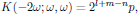
where
that is to say, for the present case of second harmonic generation

For the fundamental optical field at ω, one might be mislead to assume that since the second order interaction for this field is described by an identical set of tensor elements as for the second harmonic wave, the degeneracy factor must also be identical to the previously derived one. This is, however, a very wrong assumption, and one can easily verify that the proper degeneracy factor for the fundamental field instead is given as
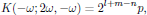
where
that is to say,

The general second harmonic polarization density of the medium is hence given as
![$$
\eqalign{
[{\bf P}^{({\rm NL})}_{2\omega}]_z&=[{\bf P}^{(2)}_{2\omega}]_z
=\varepsilon_0 \underbrace{K(-2\omega;\omega,\omega)
\chi^{(2)}_{z\alpha\beta}(-2\omega;\omega,\omega)}_{
={{1}\over{2}}\chi^{(2)}_{z\alpha\beta}(-2\omega;\omega,\omega)}
E^{\alpha}_{\omega}E^{\beta}_{\omega}\cr
&=(\varepsilon_0/2)[\chi^{(2)}_{zxx} E^x_{\omega} E^{x}_{\omega}
+\chi^{(2)}_{zyy} E^y_{\omega} E^{y}_{\omega}
+\chi^{(2)}_{zzz} E^z_{\omega} E^{z}_{\omega}]\cr
&=(\varepsilon_0/2)[\chi^{(2)}_{zxx}
(E^x_{\omega} E^{x}_{\omega}+E^y_{\omega} E^{y}_{\omega})
+\chi^{(2)}_{zzz} E^z_{\omega} E^{z}_{\omega}],\cr
[{\bf P}^{({\rm NL})}_{2\omega}]_y
&=(\varepsilon_0/2)[\chi^{(2)}_{yxx} E^x_{\omega} E^{x}_{\omega}
+\chi^{(2)}_{yyy} E^y_{\omega} E^{y}_{\omega}
+\chi^{(2)}_{yyz} E^y_{\omega} E^{z}_{\omega}
+\chi^{(2)}_{yzy} E^z_{\omega} E^{y}_{\omega}]\cr
&=(\varepsilon_0/2)[\chi^{(2)}_{yxx}
(E^x_{\omega} E^{x}_{\omega}-E^y_{\omega} E^{y}_{\omega})
+\chi^{(2)}_{zxx}
(E^y_{\omega} E^{z}_{\omega}+E^z_{\omega} E^{y}_{\omega})],\cr
[{\bf P}^{({\rm NL})}_{2\omega}]_x
&=(\varepsilon_0/2)[\chi^{(2)}_{xxy} E^x_{\omega} E^{y}_{\omega}
+\chi^{(2)}_{xyx} E^y_{\omega} E^{x}_{\omega}
+\chi^{(2)}_{xxz} E^x_{\omega} E^{z}_{\omega}
+\chi^{(2)}_{xzx} E^z_{\omega} E^{x}_{\omega}]\cr
&=(\varepsilon_0/2)[\chi^{(2)}_{yxx}
(E^x_{\omega} E^{y}_{\omega}+E^y_{\omega} E^{x}_{\omega})
+\chi^{(2)}_{zxx}
(E^x_{\omega} E^{z}_{\omega}+E^z_{\omega} E^{x}_{\omega})],\cr
}
$$](/research/lectures/lect9/web/images_80proc/lect9_eq_disp_020.png)
while the general polarization density at the angular frequency of the pump field becomes [3]
![$$
\eqalign{
[{\bf P}^{({\rm NL})}_{\omega}]_z&=[{\bf P}^{(2)}_{\omega}]_z
=\varepsilon_0 \underbrace{K(-\omega;2\omega,-\omega)
\chi^{(2)}_{z\alpha\beta}(-\omega;2\omega,-\omega)}_{
=\chi^{(2)}_{z\alpha\beta}(-2\omega;\omega,\omega)}
E^{\alpha}_{2\omega}E^{\beta}_{-\omega}\cr
&=\varepsilon_0[\chi^{(2)}_{zxx} E^x_{2\omega} E^{x*}_{\omega}
+\chi^{(2)}_{zyy} E^y_{2\omega} E^{y*}_{\omega}
+\chi^{(2)}_{zzz} E^z_{2\omega} E^{z*}_{\omega}]\cr
&=\varepsilon_0[\chi^{(2)}_{zxx}
(E^x_{2\omega} E^{x*}_{\omega}+E^y_{2\omega} E^{y*}_{\omega})
+\chi^{(2)}_{zzz} E^z_{2\omega} E^{z*}_{\omega}],\cr
[{\bf P}^{({\rm NL})}_{\omega}]_y
&=\varepsilon_0[\chi^{(2)}_{yxx} E^x_{2\omega} E^{x*}_{\omega}
+\chi^{(2)}_{yyy} E^y_{2\omega} E^{y*}_{\omega}
+\chi^{(2)}_{yyz} E^y_{2\omega} E^{z*}_{\omega}
+\chi^{(2)}_{yzy} E^z_{2\omega} E^{y*}_{\omega}]\cr
&=\varepsilon_0[\chi^{(2)}_{yxx}
(E^x_{2\omega} E^{x*}_{\omega}-E^y_{2\omega} E^{y*}_{\omega})
+\chi^{(2)}_{zxx}
(E^y_{2\omega} E^{z*}_{\omega}+E^z_{2\omega} E^{y*}_{\omega})],\cr
[{\bf P}^{({\rm NL})}_{\omega}]_x
&=\varepsilon_0[\chi^{(2)}_{xxy} E^x_{2\omega} E^{y*}_{\omega}
+\chi^{(2)}_{xyx} E^y_{2\omega} E^{x*}_{\omega}
+\chi^{(2)}_{xxz} E^x_{2\omega} E^{z*}_{\omega}
+\chi^{(2)}_{xzx} E^z_{2\omega} E^{x*}_{\omega}]\cr
&=\varepsilon_0[\chi^{(2)}_{yxx}
(E^x_{2\omega} E^{y*}_{\omega}+E^y_{2\omega} E^{x*}_{\omega})
+\chi^{(2)}_{zxx}
(E^x_{2\omega} E^{z*}_{\omega}+E^z_{2\omega} E^{x*}_{\omega})].\cr
}
$$](/research/lectures/lect9/web/images_80proc/lect9_eq_disp_022.png)
For a pump wave polarized in the yz-plane of the crystal frame, the polarization density of the medium hence becomes
![$$
\eqalign{
[{\bf P}^{({\rm NL})}_{2\omega}]_z
&=(\varepsilon_0/2)[\chi^{(2)}_{zxx}
E^y_{\omega} E^y_{\omega}
+\chi^{(2)}_{zzz} E^z_{\omega} E^{z}_{\omega}],\cr
[{\bf P}^{({\rm NL})}_{2\omega}]_y
&=(\varepsilon_0/2)[-\chi^{(2)}_{yxx} E^y_{\omega} E^{y}_{\omega}
+\chi^{(2)}_{zxx}
(E^y_{\omega} E^{z}_{\omega}+E^z_{\omega} E^{y}_{\omega})],\cr
[{\bf P}^{({\rm NL})}_{2\omega}]_x
&=0,\cr
}
$$](/research/lectures/lect9/web/images_80proc/lect9_eq_disp_023.png)
and
![$$
\eqalign{
[{\bf P}^{({\rm NL})}_{\omega}]_z
&=\varepsilon_0[\chi^{(2)}_{zxx} E^y_{2\omega} E^{y*}_{\omega}
+\chi^{(2)}_{zzz} E^z_{2\omega} E^{z*}_{\omega}],\cr
[{\bf P}^{({\rm NL})}_{\omega}]_y
&=\varepsilon_0[-\chi^{(2)}_{yxx}E^y_{2\omega} E^{y*}_{\omega}
+\chi^{(2)}_{zxx}
(E^y_{2\omega} E^{z*}_{\omega}+E^z_{2\omega} E^{y*}_{\omega})],\cr
[{\bf P}^{({\rm NL})}_{\omega}]_x
&=0.\cr
}
$$](/research/lectures/lect9/web/images_80proc/lect9_eq_disp_024.png)
3.5. The wave equation
Strictly speaking, the previously formulated polarization density gives a coupled system between the polarization states of both the fundamental and second harmonic waves, since both the y- and z-components of the polarization densities at ω and 2ω contain components of all other field components. However, for simplicity we will here restrict the continued analysis to the case of a y-polarized input pump wave, which through the χ(2)zyy = χ(2)zxx elements give rise to a z-polarized second harmonic frequency component at 2ω.
The electric fields of the fundamental and second harmonic optical waves are for the forward propagating configuration expressed in their spatial envelopes Aω and A2ω as

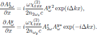
Using the above separation of the natural, spatial oscillation of the light, in the infinite plane wave approximation and by using the slowly varying envelope approximation, the wave equation for the envelope of the second harmonic optical field becomes (see Eq. (6) in lecture eight)
![$$
\eqalign{
{{\partial A^z_{2\omega}}\over{\partial x}}
&=i{{\mu_0(2\omega)^2}\over{2k_{2\omega_z}}}
[{\bf P}^{({\rm NL})}_{2\omega}]_z
\exp(-ik_{2\omega_z}x)\cr
&=i{{\mu_0(2\omega)^2}\over{2(2\omega n_{2\omega_z}/c)}}
\underbrace{
{{\varepsilon_0}\over{2}}
\chi^{(2)}_{zxx} A^y_{\omega}{}^2\exp(2ik_{\omega_y}x)}_{
=[{\bf P}^{({\rm NL})}_{2\omega}]_z}
\exp(-ik_{2\omega_z}x)\cr
&=i{{\omega\chi^{(2)}_{zxx}}\over{2 n_{2\omega_z} c}}
A^y_{\omega}{}^2\exp[i(2k_{\omega_y}-k_{2\omega_z})x],\cr
}
$$](/research/lectures/lect9/web/images_80proc/lect9_eq_disp_026.png)
while for the fundamental wave,
![$$
\eqalign{
{{\partial A^y_{\omega}}\over{\partial x}}
&=i{{\mu_0 \omega^2}\over{2k_{\omega_y}}}
[{\bf P}^{({\rm NL})}_{\omega}]_y
\exp(-ik_{\omega_y}x)\cr
&=i{{\mu_0 \omega^2}\over{2(\omega n_{\omega_y}/c)}}
\underbrace{\varepsilon_0\chi^{(2)}_{zxx}
A^z_{2\omega}\exp(ik_{2\omega_z}x)
A^{y*}_{\omega}\exp(-ik_{\omega_y}x)}_{
=[{\bf P}^{({\rm NL})}_{\omega}]_y}
\exp(-ik_{\omega_y}x)\cr
&=i{{\omega\chi^{(2)}_{zxx}}\over{2 n_{\omega_y} c}}
A^z_{2\omega}A^{y*}_{\omega}
\exp[-i(2k_{\omega_y}-k_{2\omega_z})x].\cr
}
$$](/research/lectures/lect9/web/images_80proc/lect9_eq_disp_027.png)
These equations can hence be summarized by the coupled system
where
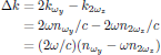
is the phase mismatch between the pump and second harmonic wave. In the case of perfect phase-matching, Δk = 0.
3.6. Boundary conditions
Here the boundary conditions are simply that no second harmonic signal is present at the input,

together with a known input field at the fundamental frequency,

3.7. Solving the wave equation
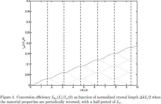
Considering a nonzero Δk, the conversion efficiency is regularly quite small, and one may approximately take the spatial distribution of the pump wave to be constant, Ayω(x) ≈ Ayω(0)$. Using this approximation [4], and by applying the initial condition Az2ω(0) = 0 of the second harmonic signal, one finds
![$$
\eqalign{
A^z_{2\omega}(L)
&=\int^L_0{{\partial A^z_{2\omega}(z)}\over{\partial x}}\,dx\cr
&=\int^L_0 i{{\omega\chi^{(2)}_{zxx}}\over{2 n_{{2\omega}_z}} c}
A^y_{\omega}{}^2(0)\exp(i\Delta k x)\,dx\cr
&={{\omega\chi^{(2)}_{zxx}}\over{2 n_{{2\omega}_z}} c}
A^y_{\omega}{}^2(0){{1}\over{\Delta k}}[\exp(i\Delta k L)-1]\cr
&=\big\{{\rm Use\ }[\exp(i\Delta k L)-1]/\Delta k
=iL\exp(i\Delta k L/2)\sinc(\Delta k L/2)\big\}\cr
&=i{{\omega\chi^{(2)}_{zxx} L}\over{2 n_{{2\omega}_z}} c}
A^y_{\omega}{}^2(0)\exp(i\Delta k L/2)\sinc(\Delta k L/2).\cr
}
$$](/research/lectures/lect9/web/images_80proc/lect9_eq_disp_032.png)
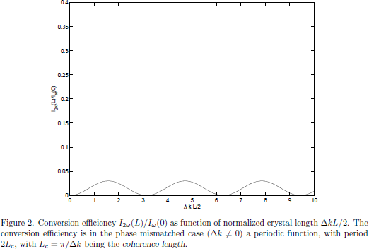
In terms if the light intensities of the waves, one after a propagation distance x = L hence has the second harmonic signal with intensity I2ω(L) expressed in terms of the input intensity Iω(L) expressed in terms of as
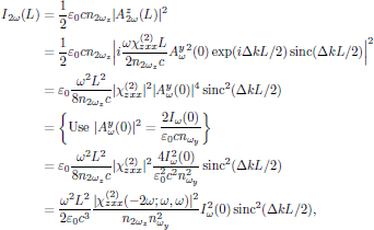
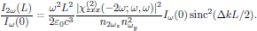
that is to say, with the conversion efficiency
4. Optical Kerr-effect - Field corrected refractive index
As a start, we assume a monochromatic optical wave (containing forward and/or backward propagating components) polarized in the xy-plane,
![$$
{\bf E}(z,t)=\Re[{\bf E}_{\omega}(z)\exp(-i\omega t)]\in{\Bbb R}^3,
$$](/research/lectures/lect9/web/images_80proc/lect9_eq_disp_035.png)
with all spatial variation of the field contained in

4.1. The optical interaction
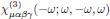
Optical Kerr-effect is in isotropic media described by the third order susceptibility [5]
4.2. Symmetries of the medium
The general set of nonzero components of χ(3)μαβγ for isotropic media are from Appendix A3.3 of Butcher and Cotters book given as
 (3)
(3)with

that is to say, a general set of 21 elements, of which only 3 are independent.
4.3. Additional symmetries
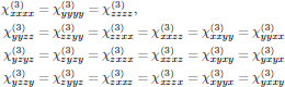
By applying the intrinsic permutation symmetry in the middle indices for optical Kerr-effect, one generally has

which hence slightly reduces the set (3) to still 21 nonzero elements, but of which now only two are independent. For a beam polarized in the xy-plane, the elements of interest are only those which only contain x or y in the indices, that is to say, the subset

with

that is to say, a set of eight elements, of which only two are independent.
4.4. The polarization density
The degeneracy factor K(-ω;ω,ω,-ω) is calculated as

From the reduced set of nonzero susceptibilities for the beam polarized in the xy-plane, and by using the calculated value of the degeneracy factor in the convention of Butcher and Cotter, we hence have the third order electric polarization density at ωσ =ω given as
![${\bf P}^{(n)}({\bf r},t)=\Re[{\bf P}^{(n)}_{\omega}\exp(-i\omega t)]$](/research/lectures/lect9/web/images_80proc/lect9_eq_inline_006.png)
with
![$$
\eqalign{
{\bf P}^{(3)}_{\omega}
&=\sum_{\mu}{\bf e}_{\mu}(P^{(3)}_{\omega})_{\mu}\cr
&=\{{\rm Using\ the\ convention\ of\ Butcher\ and\ Cotter}\}\cr
&=\sum_{\mu}{\bf e}_{\mu}
\bigg[\varepsilon_0{{3}\over{4}}\sum_{\alpha}\sum_{\beta}\sum_{\gamma}
\chi^{(3)}_{\mu\alpha\beta\gamma}(-\omega;\omega,\omega,-\omega)
(E_{\omega})_{\alpha}(E_{\omega})_{\beta}(E_{-\omega})_{\gamma}\bigg]\cr
&=\{{\rm Evaluate\ the\ sums\ over\ } (x,y,z)
{\rm\ for\ field\ polarized\ in\ the\ }xy{\rm\ plane}\}\cr
&=\varepsilon_0{{3}\over{4}}\{
{\bf e}_x[
\chi^{(3)}_{xxxx} E^x_{\omega} E^x_{\omega} E^x_{-\omega}
+\chi^{(3)}_{xyyx} E^y_{\omega} E^y_{\omega} E^x_{-\omega}
+\chi^{(3)}_{xyxy} E^y_{\omega} E^x_{\omega} E^y_{-\omega}
+\chi^{(3)}_{xxyy} E^x_{\omega} E^y_{\omega} E^y_{-\omega}]\cr
&\qquad\quad
+{\bf e}_y[
\chi^{(3)}_{yyyy} E^y_{\omega} E^y_{\omega} E^y_{-\omega}
+\chi^{(3)}_{yxxy} E^x_{\omega} E^x_{\omega} E^y_{-\omega}
+\chi^{(3)}_{yxyx} E^x_{\omega} E^y_{\omega} E^x_{-\omega}
+\chi^{(3)}_{yyxx} E^y_{\omega} E^x_{\omega} E^x_{-\omega}]\}\cr
&=\{{\rm Make\ use\ of\ }{\bf E}_{-\omega}={\bf E}^*_{\omega}
{\rm\ and\ relations\ }\chi^{(3)}_{xxyy}=\chi^{(3)}_{yyxx},
{\rm\ etc.}\}\cr
&=\varepsilon_0{{3}\over{4}}\{
{\bf e}_x[
\chi^{(3)}_{xxxx} E^x_{\omega} |E^x_{\omega}|^2
+\chi^{(3)}_{xyyx} E^y_{\omega}{}^2 E^{x*}_{\omega}
+\chi^{(3)}_{xyxy} |E^y_{\omega}|^2 E^x_{\omega}
+\chi^{(3)}_{xxyy} E^x_{\omega} |E^y_{\omega}|^2]\cr
&\qquad\quad
+{\bf e}_y[
\chi^{(3)}_{xxxx} E^y_{\omega} |E^y_{\omega}|^2
+\chi^{(3)}_{xyyx} E^x_{\omega}{}^2 E^{y*}_{\omega}
+\chi^{(3)}_{xyxy} |E^x_{\omega}|^2 E^y_{\omega}
+\chi^{(3)}_{xxyy} E^y_{\omega} |E^x_{\omega}|^2]\}\cr
&=\{{\rm Make\ use\ of\ the\ intrinsic\ permutation\ symmetry}\}\cr
&=\varepsilon_0{{3}\over{4}}\{
{\bf e}_x[
(\chi^{(3)}_{xxxx} |E^x_{\omega}|^2
+2\chi^{(3)}_{xxyy} |E^y_{\omega}|^2) E^x_{\omega}
+(\chi^{(3)}_{xxxx}-2\chi^{(3)}_{xxyy})
E^y_{\omega}{}^2 E^{x*}_{\omega}\cr
&\qquad\quad
{\bf e}_y[
(\chi^{(3)}_{xxxx} |E^y_{\omega}|^2
+2\chi^{(3)}_{xxyy} |E^x_{\omega}|^2) E^y_{\omega}
+(\chi^{(3)}_{xxxx}-2\chi^{(3)}_{xxyy})
E^x_{\omega}{}^2 E^{y*}_{\omega}.\cr
}
$$](/research/lectures/lect9/web/images_80proc/lect9_eq_disp_046.png)
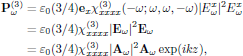
For the optical field being linearly polarized, say in the x-direction, the expression for the polarization density is significantly simplified, to yield

that is to say, taking a form that can be interpreted as an intensity-dependent (∼|Exω|2) contribution to the refractive index (see Butcher and Cotter §6.3.1).
4.5. The wave equation - Time independent case
In this example, we consider continuous wave propagation (That is to say, a time independent problem with the temporal envelope of the electrical field being constant in time) in optical Kerr-media, using light polarized in the x-direction and propagating along the positive direction of the z-axis,
![$$
{\bf E}({\bf r},t)=\Re[{\bf E}_{\omega}(z)\exp(-i\omega t)],
\qquad{\bf E}_{\omega}(z)={\bf A}_{\omega}(z)\exp(ikz)
={\bf e}_x A^x_{\omega}(z)\exp(ikz),
$$](/research/lectures/lect9/web/images_80proc/lect9_eq_disp_048.png)
where, as previously, k = ωn0/c. From material handed out during the third lecture (notes on the Butcher and Cotter convention), the nonlinear polarization density for x-polarized light is given as

with
and the time independent wave equation for the field envelope Aω, again using Eq. (6) of lecture eight, becomes
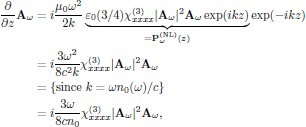
or, equivalently, in its scalar form
4.6. Boundary conditions - Time independent case
For this special case of unidirectional wave propagation, the boundary condition is simply a known optical field at the input,

4.7. Solving the wave equation - Time independent case
If the medium of interest now is analyzed at an angular frequency far from any resonance, we may look for solutions to this equation with |Aω(z)| being constant (for a lossless medium). For such a case it is straightforward to integrate the final wave equation to yield the general solution
![$$
{\bf A}_{\omega}(z)={\bf A}_{\omega}(0)
\exp[i{{3\omega}\over{8cn_0}}\chi^{(3)}_{xxxx}|{\bf A}_{\omega}(0)|^2 z],
$$](/research/lectures/lect9/web/images_80proc/lect9_eq_disp_053.png)
or, again equivalently, in the scalar form
![$$
A^x_{\omega}(z)=
A^x_{\omega}(0)
\exp[i{{3\omega}\over{8cn_0}}\chi^{(3)}_{xxxx}|A^x_{\omega}(0)|^2 z],
$$](/research/lectures/lect9/web/images_80proc/lect9_eq_disp_054.png)
which hence gives the solution for the real-valued electric field E(r,t) as
![$$
\eqalign{
{\bf E}({\bf r},t)&=\Re[{\bf E}_{\omega}(z)\exp(-i\omega t)]\cr
&=\Re\{{\bf A}_{\omega}(z)\exp[i(kz-\omega t)]\}\cr
&=\Re\{{\bf A}_{\omega}(0)
\exp[i(\underbrace{{{\omega n_0}\over{c}}z
+{{3\omega}\over{8cn_0}}\chi^{(3)}_{xxxx}|A^x_{\omega}(0)|^2 z}_{
\equiv k_{\rm eff}z}
-\omega t)]\}.\cr
}
$$](/research/lectures/lect9/web/images_80proc/lect9_eq_disp_055.png)
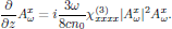
From this solution, one immediately finds that the wave propagates with an effective propagation constant
![$$
k_{\rm eff}={{\omega}\over{c}}
[n_0+{{3}\over{8n_0}}\chi^{(3)}_{xxxx}|A^x_{\omega}(0)|^2],
$$](/research/lectures/lect9/web/images_80proc/lect9_eq_disp_056.png)
that is to say, experiencing the intensity dependent refractive index
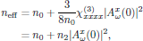
with

10. References
[1] Keep in mind that in the convention of Butcher and Cotter, the frequency arguments to the right of the semicolon may be writen in arbitrary order, hence we may in an equal description instead use

for the description of the second order interaction between light and matter.
[2] See course material on the Butcher and Cotter convention, handed out during the third lecture. Notice that for the first order polarization density, one at optical frequencies always has the trivial degeneracy factor

[3] Keep in mind that a negative frequency argument to the right of the semicolon in the susceptibility is to be associated with the complex conjugate of the respective electric field; see Butcher and Cotter, section 2.3.2.
[4]
For an outline of the method of
solving the coupled system exactly in terms of Jacobian elliptic
functions (thus allowing for a depleted pump as well), see one of the
pioneering works in nonlinear optics by J. A. Armstrong,
N. Bloembergen, J. Ducuing, and P. S. Pershan, Interactions between Light
Waves in a Nonlinear Dielectric
Phys. Rev.
127, 1918-1939, (1962).
DOI: 10.1103/PhysRev.127.1918
[5] Again, keep in mind that in the convention of Butcher and Cotter, the frequency arguments to the right of the semicolon may be writen in arbitrary order, hence we may in an equal description instead use
or
for this description of the third order interaction between light and matter.