Lectures on Nonlinear Optics - Lecture 8

The nonlinear electromagnetic wave equation

lect8.pdf [151 kB] Lecture 8 in Portable Document Format.

In this lecture, the electric polarisation density of the medium is finally inserted into Maxwell's equations, and the wave propagation properties of electromagnetic waves in nonlinear optical media is for the first time in this course analysed. As an example of wave propagation in nonlinear optical media, the optical Kerr effect is analysed for infinite plane continuous waves.

The outline for this lecture is:

Maxwells equations (general electromagnetic wave propagation).
Time dependent processes (envelopes slowly varying in space and time).
Time independent processes (envelopes slowly varying in space but constant in time).
Examples (Optical Kerr-effect ↔ χ⁽³⁾_μαβγ(−ω; ω, ω, −ω)).

1. Wave propagation in nonlinear media

1.1. Maxwell's equations

The propagation of electromagnetic waves are, from a first principles approach, governed by the Maxwell's equations (here listed in their real-valued form in SI units),

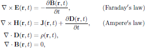
$\eqalign{ \nabla\times {\bf E}({\bf r},t) &= -{{\partial{\bf B}({\bf r},t)}\over{\partial{t}}},\hskip 50pt ({\textstyle\rm Faraday's\ law})\cr \nabla\times{\bf H}({\bf r},t) &= {\bf J}({\bf r},t) + {{\partial{\bf D}({\bf r},t)}\over{\partial{t}}},\hskip 18.7pt ({\textstyle\rm Ampere's\ law})\cr \nabla\cdot{\bf D}({\bf r},t)&=\rho({\bf r},t),\cr \nabla\cdot{\bf B}({\bf r},t)&=0,\cr }$

where ρ(r,t) is the density of free charges and J(r,t) the corresponding current density of free charges.

1.2. Constitutive relations

The constitutive relations are in SI units formulated as

$\eqalign{ {\bf D}({\bf r},t)&=\varepsilon_0{\bf E}({\bf r},t)+{\bf P}({\bf r},t),\cr {\bf B}({\bf r},t)&=\mu_0[{\bf H}({\bf r},t) + {\bf M}({\bf r},t)],\cr }$

where P(r,t) = P[E(r,t), B(r,t)] is the macroscopic polarization density (electric dipole moment per unit volume) and M(r,t) = M[E(r,t), B(r,t)] the magnetization (magnetic dipole moment per unit volume) of the medium.

Here E(r,t) and B(r,t) are considered as the fundamental macroscopic electric and magnetic field quantities; D(r,t) and H(r,t) are the corresponding derived fields associated with the state of matter, connected to E(r,t) and B(r,t) through the electric polarization density P(r,t) and magnetization (magnetic polarization density) M(r,t) through the basic constitutive relations. In fact, the constitutive equations above form the very definitions [1, 2] of the electric polarization density and magnetization.

2. Two frequent assumptions in nonlinear optics

No free charges present,
$\rho({\bf r},t)=0,\qquad{\bf J}({\bf r},t)={\bf 0}.$
(Any relaxation processes are included in imaginary parts of the terms of the electric susceptibility.)
No magnetization of the medium,
${\bf M}({\bf r},t)={\bf 0}.$

3. The wave equation

By taking the cross product with the nabla operator and Faraday's law, one obtains

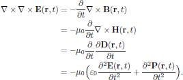
$\eqalign{ \nabla\times\nabla\times{\bf E}({\bf r},t) &=-{{\partial}\over{\partial{t}}}\nabla\times{\bf B}({\bf r},t)\cr &=-\mu_0{{\partial}\over{\partial{t}}}\nabla\times{\bf H}({\bf r},t)\cr &=-\mu_0{{\partial}\over{\partial{t}}} {{\partial{\bf D}({\bf r},t)}\over{\partial t}}\cr &=-\mu_0\Big( \varepsilon_0{{\partial^2{\bf E}({\bf r},t)}\over{\partial t^2}} +{{\partial^2{\bf P}({\bf r},t)}\over{\partial t^2}}\Big).\cr }$

Since μ₀ε₀ = 1/c² in SI units, with c being the speed of light in vacuum, one hence obtains the basic wave equation, taken in time domain, as

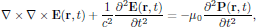$\nabla\times\nabla\times{\bf E}({\bf r},t) +{{1}\over{c^2}}{{\partial^2{\bf E}({\bf r},t)}\over{\partial t^2}} =-\mu_0{{\partial^2{\bf P}({\bf r},t)}\over{\partial t^2}},\eqno{(1)}$ (1)

where, as in the previous lectures of this course, the polarization density can be written in terms of the perturbation series as

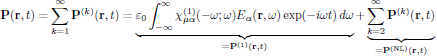
$\eqalign{ {\bf P}({\bf r},t)&=\sum^{\infty}_{k=1}{\bf P}^{(k)}({\bf r},t) =\underbrace{ \varepsilon_0\int^{\infty}_{-\infty} \chi^{(1)}_{\mu\alpha}(-\omega;\omega) E_{\alpha}({\bf r},\omega)\exp(-i\omega t)\,d\omega }_{={\bf P}^{(1)}({\bf r},t)} +\underbrace{ \sum^{\infty}_{k=2}{\bf P}^{(k)}({\bf r},t) }_{={\bf P}^{({\rm NL})}({\bf r},t)}\cr }$

In the left hand side of Eq. (1), we find the part of the homogeneous wave equation for propagation of electromagnetic waves in vacuum, while the right hand side described the modifications to the vacuum propagation due to the interaction between light and matter. In this respect, it is now clear that the electric polarisation effectively acts as a source term in the mathematical description of electromagnetic wave propagation, making the otherwise homogeneous vacuum problem an inhomogeneous problem (though with known source terms).

It should be noticed that whenever the polarization density is calculated from the Bloch equations (formulated later on, in lecture 10 of this course), instead of by means of a perturbation series as above, the Maxwell equations and the wave equation (1) above are denoted Maxwell-Bloch equations. In some sense, we can therefore see the choice of method for the calculation of the polarization density as a switch point not only for using the susceptibility formalism or not for the description of interaction between light and matter, but also for the form of the wave propagation problem in nonlinear media, which mathematically significantly differ between the "pure" Maxwell's equations with susceptibilities and the Maxwell-Bloch equations.

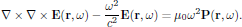
4. The wave equation in frequency domain (optional)

Frequently in this course, we have rather been studying the electric fields and polarisation densities in frequency domain, since many phenomena in optics are properly and conveniently described as static (in which case the frequency dependence is simply reduced to the interaction between discrete frequencies in the spectrum). By using the Fourier integral identity [3]

$E_{\alpha}(t)=\int^{\infty}_{-\infty}E_{\alpha}(\omega) \exp(-i\omega t)\,d\omega=\fourier^{-1}[E_{\alpha}](t),$

with inverse relation

$E_{\alpha}(\omega)={{1}\over{2\pi}}\int^{\infty}_{-\infty}E_{\alpha}(\tau) \exp(i\omega\tau)\,d\tau=\fourier[E_{\alpha}](\omega),$

we obtain the wave equation (1) as

$\nabla\times\nabla\times{\bf E}({\bf r},\omega) -{{\omega^2}\over{c^2}}{\bf E}({\bf r},\omega) =\mu_0\omega^2{\bf P}({\bf r},\omega).$

5. Quasimonochromatic light - Time dependent problems

By inserting the perturbation series for the electric polarisation density into the general wave equation (1), which apply to arbitrary electric field distributions and field intensities of the light, one obtains the equation

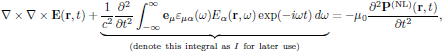$\nabla\times\nabla\times{\bf E}({\bf r},t) +\underbrace{{{1}\over{c^2}}{{\partial^2}\over{\partial t^2}} \int^{\infty}_{-\infty}{\bf e}_{\mu}\varepsilon_{\mu\alpha}(\omega) E_{\alpha}({\bf r},\omega)\exp(-i\omega t)\,d\omega }_{({\rm denote\ this\ integral\ as\ }I{\rm\ for\ later\ use})} =-\mu_0{{\partial^2{\bf P}^{({\rm NL})}({\bf r},t)}\over{\partial t^2}}, \eqno{(2)}$ (2)

where

$\varepsilon_{\mu\alpha}(\omega)=\delta_{\mu\alpha} +\chi^{(1)}_{\mu\alpha}(-\omega;\omega)$

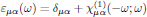
is a parameter commonly denoted as the relative electrical permittivity [4]. (This wave equation is identical to Eq. (7.14) in Butcher and Cotter's book. Notice though the printing error in Butcher and Cotter's Eq. (7.14), where the first μ₀ should be replaced by 1/c².)

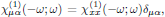
The second term of the left hand side of Eq. (2) provides all first order optical contributions to the wave propagation, as well as all linear optical dispersion effects. This terms deserves some extra attention, and we will now proceed with deriving the effect of the frequency dependence of the relative permittivity upon the wave equation. First of all, we notice that since E_α(r,−ω) = E_α^*(r,ω), which simply is a consequence of the choice of complex Fourier transform of a real valued field, the reality condition of Eq. (2) requires that

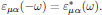
$\varepsilon_{\mu\alpha}(-\omega)=\varepsilon^*_{\mu\alpha}(\omega).$

It should be emphasized that this property of the relative electrical permittivity merely is a convenient mathematical construction, since we in regular physical terms only consider positive angular frequencies as argument for the refractive index, etc.

For quasimonochromatic light, the electric field and polarisation density are taken as

$\eqalign{ {\bf E}({\bf r},t)&=\sum_{\omega_{\sigma}\ge 0} \Re[{\bf E}_{\omega_{\sigma}}({\bf r},t)\exp(-i\omega_{\sigma} t)],\cr {\bf P}({\bf r},t)&=\sum_{\omega_{\sigma}\ge 0} \Re[{\bf P}_{\omega_{\sigma}}({\bf r},t)\exp(-i\omega_{\sigma} t)],\cr }$

where E_{ω_σ}(r,t) and P_{ω_σ}(r,t) are slowly varying envelopes of the fields. In the frequency domain, the quasimonochromatic fields are expressed as

$\eqalign{ {\bf E}({\bf r},\omega)&={{1}\over{2}}\sum_{\omega_{\sigma}\ge 0} [{\bf E}_{\omega_{\sigma}}({\bf r},\omega-\omega_{\sigma}) +{\bf E}^*_{\omega_{\sigma}}({\bf r},-\omega-\omega_{\sigma})],\cr {\bf P}({\bf r},\omega)&={{1}\over{2}}\sum_{\omega_{\sigma}\ge 0} [{\bf P}_{\omega_{\sigma}}({\bf r},\omega-\omega_{\sigma}) +{\bf P}^*_{\omega_{\sigma}}({\bf r},-\omega-\omega_{\sigma})],\cr }$

where the envelopes have some limited extent around the carrier frequencies at ±ω_σ. Notice that the fields taken in the frequency domain are expressed entirely in terms of their respective temporal envelope, that is to say, without the exponential functions that appear in their counterparts in time domain.

For simplicity considering a medium that in the linear optical domain is isotropic, with the relative electrical permittivity

$\varepsilon_{\mu\alpha}(\omega) =\varepsilon(\omega)\delta_{\mu\alpha} =n^2_0(\omega)\delta_{\mu\alpha},$

where n₀(ω) is the first order contribution to the refractive index of the medium, this leads to the middle term of the wave equation (1) in the form

$\eqalign{ I&\equiv{{1}\over{c^2}}{{\partial^2}\over{\partial t^2}} \int^{\infty}_{-\infty}{\bf e}_{\mu}\varepsilon_{\mu\alpha}(\omega) E_{\alpha}({\bf r},\omega)\exp(-i\omega t)\,d\omega\cr &=-\int^{\infty}_{-\infty}{{\omega^2 n^2(\omega)}\over{c^2}} \underbrace{ {{1}\over{2}}\sum_{\omega_{\sigma}\ge 0} [{\bf E}_{\omega_{\sigma}}({\bf r},\omega-\omega_{\sigma}) +{\bf E}^*_{\omega_{\sigma}}({\bf r},-\omega-\omega_{\sigma})]}_{ {\rm quasimonochromatic\ form\ of\ }{\bf E}({\bf r},\omega)} \exp(-i\omega t)\,d\omega\cr &=\{{\rm denote\ }\omega^2\varepsilon(\omega)/c^2 \equiv\omega^2 n^2_0(\omega)/c^2\equiv k^2(\omega)\}\cr &=-{{1}\over{2}}\sum_{\omega_{\sigma}\ge 0} \int^{\infty}_{-\infty}k^2(\omega) [{\bf E}_{\omega_{\sigma}}({\bf r},\omega-\omega_{\sigma}) +{\bf E}^*_{\omega_{\sigma}}({\bf r},-\omega-\omega_{\sigma})] \exp(-i\omega t)\,d\omega.\cr &=-{{1}\over{2}}\sum_{\omega_{\sigma}\ge 0} \int^{\infty}_{-\infty}k^2(\omega) {\bf E}_{\omega_{\sigma}}({\bf r},\omega-\omega_{\sigma}) \exp(-i\omega t)\,d\omega + {\rm c.\,c.}\cr }$

If now the field envelopes decay to zero rapidly enough in the vicinity of the carrier frequencies (as we would expect for quasimonochromatic light, with a strong spectral confinement around the carrier frequency of the light), then we may expect that a good approximation is to make a Taylor expansion of $k^2(\omega)$, in the neighbourhood of respective carrier frequency of the light, as

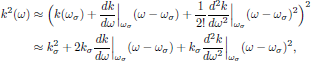
$\eqalign{ k^2(\omega)&\approx\Big(k(\omega_{\sigma}) +{{dk}\over{d\omega}}\Big|_{\omega_{\sigma}}(\omega-\omega_{\sigma}) +{{1}\over{2!}}{{d^2 k}\over{d\omega^2}} \Big|_{\omega_{\sigma}}(\omega-\omega_{\sigma})^2 \Big)^2\cr &\approx k^2_{\sigma} +2k_{\sigma}{{dk}\over{d\omega}} \Big|_{\omega_{\sigma}}(\omega-\omega_{\sigma}) +k_{\sigma}{{d^2 k}\over{d\omega^2}} \Big|_{\omega_{\sigma}}(\omega-\omega_{\sigma})^2, \cr }$

where the notation k_σ = k(ω_σ) was introduced, and hence [5]

$\eqalign{ I&\approx -{{1}\over{2}}\sum_{\omega_{\sigma}\ge 0}\int^{\infty}_{-\infty} \Big(k^2_{\sigma} +2k_{\sigma}{{dk}\over{d\omega}} \Big|_{\omega_{\sigma}}(\omega-\omega_{\sigma}) +k_{\sigma}{{d^2 k}\over{d\omega^2}} \Big|_{\omega_{\sigma}}(\omega-\omega_{\sigma})^2 \Big) \cr&\qquad\qquad\qquad\qquad\qquad\qquad\qquad\qquad\times {\bf E}_{\omega_{\sigma}}({\bf r},\omega-\omega_{\sigma}) \exp(-i\omega t)\,d\omega + {\rm c.\,c.}\cr &=\{{\rm change\ variable\ of\ integration\ } \omega'=\omega-\omega_{\sigma}\}\cr &=-{{1}\over{2}}\sum_{\omega_{\sigma}\ge 0}\int^{\infty}_{-\infty} \Big(k^2_{\sigma} +2k_{\sigma}{{dk}\over{d\omega}} \Big|_{\omega_{\sigma}}\omega' +k_{\sigma}{{d^2 k}\over{d\omega^2}} \Big|_{\omega_{\sigma}}\omega'^2 \Big) \cr&\qquad\qquad\qquad\qquad\qquad\qquad\qquad\qquad\times {\bf E}_{\omega_{\sigma}}({\bf r},\omega') \exp(-i\omega't)\,d\omega'\,\exp(-i\omega_{\sigma} t) + {\rm c.\,c.}\cr &=\bigg\{{\rm use\ }\int^{\infty}_{-\infty}\omega^n f(\omega) \exp(-i\omega t)\,d\omega=\fourier^{-1}[\omega^n f(\omega)](t) =i^n{{d^n f(t)}\over{d t^n}}\bigg\}\cr &=-{{1}\over{2}}\sum_{\omega_{\sigma}\ge 0}\exp(-i\omega_{\sigma} t) \Big(k^2_{\sigma} +i2k_{\sigma}{{dk}\over{d\omega}} \Big|_{\omega_{\sigma}}{{\partial}\over{\partial t}} -k_{\sigma}{{d^2 k}\over{d\omega^2}} \Big|_{\omega_{\sigma}}{{\partial^2}\over{\partial t^2}} \Big){\bf E}_{\omega_{\sigma}}({\bf r},t) + {\rm c.\,c.}\cr }$

As this result is inserted back into the wave equation (2), one obtains

$\eqalign{ {{1}\over{2}}\sum_{\omega_{\sigma}\ge 0}&\exp(-i\omega_{\sigma} t) \Big[\nabla\times\nabla\times{\bf E}_{\omega_{\sigma}}({\bf r},t) \cr&\qquad\qquad\qquad -\Big(k^2_{\sigma} +2ik_{\sigma}{{dk}\over{d\omega}} \Big|_{\omega_{\sigma}}{{\partial}\over{\partial t}} -k_{\sigma}{{d^2 k}\over{d\omega^2}} \Big|_{\omega_{\sigma}}{{\partial^2}\over{\partial t^2}} \Big){\bf E}_{\omega_{\sigma}}({\bf r},t)\Big] + {\rm c.\,c.}\cr &=-\mu_0{{\partial^2{\bf P}^{({\rm NL})}({\bf r},t)} \over{\partial t^2}}\cr &=-\mu_0{{\partial^2}\over{\partial t^2}} {{1}\over{2}} \sum_{\omega_{\sigma}\ge 0} {\bf P}^{({\rm NL})}_{\omega_{\sigma}}({\bf r},t) \exp(-i\omega_{\sigma} t)+{\rm c.\,c.}\cr &\approx\mu_0{{1}\over{2}}\sum_{\omega_{\sigma}\ge 0}\omega^2_{\sigma} {\bf P}^{({\rm NL})}_{\omega_{\sigma}}({\bf r},t) \exp(-i\omega_{\sigma} t)+{\rm c.\,c.}\cr }$

As we separate out the respective frequency components at ω = ω_σ of this equation, one obtains the time dependent wave equation for the temporal envelope components of the electric field as

$\eqalign{ \nabla\times\nabla\times{\bf E}_{\omega_{\sigma}}({\bf r},t) -\Big(k^2_{\sigma} +i2k_{\sigma} {{1}\over{v_{\rm g}}} {{\partial}\over{\partial t}} -k_{\sigma}{{d^2 k}\over{d\omega^2}}& \Big|_{\omega_{\sigma}}{{\partial^2}\over{\partial t^2}} \Big){\bf E}_{\omega_{\sigma}}({\bf r},t) =\mu_0\omega^2_{\sigma} {\bf P}^{({\rm NL})}_{\omega_{\sigma}}({\bf r},t),\cr } \eqno{(3)}$ (3)

where

$v_{\rm g}=\Big({{dk}\over{d\omega}}\Big|_{\omega_{\sigma}}\Big)^{-1}.$

is the group velocity.

6. Three practical approximations

The infinite plane wave approximation,
${\bf E}_{\omega_{\sigma}}({\bf r},t) ={\bf E}_{\omega_{\sigma}}(z,t)\bot{\bf e}_z \qquad\Rightarrow\qquad \nabla\times\nabla\times\to -{{\partial^2}\over{\partial z^2}}.$
Unidirectional propagation,
$\eqalign{ {\bf E}_{\omega_{\sigma}}(z,t)&={\bf A}_{\omega_{\sigma}}(z,t) \exp(\pm ik_{\sigma}z)\cr &\Downarrow\cr \nabla\times\nabla\times{\bf E}_{\omega_{\sigma}}(z,t)&= -[{{\partial^2{\bf A}_{\omega_{\sigma}}}\over{\partial z^2}} \pm 2ik_{\sigma}{{\partial{\bf A}_{\omega_{\sigma}}}\over{\partial z}} -k^2_{\sigma}{\bf A}_{\omega_{\sigma}} ]\exp(\pm ik_{\sigma}z),\cr }$
for waves propagating in the positive/negative z-direction. In this case, the real-valued electric field hence takes the form
$\eqalign{ {\bf E}({\bf r},t)&=\sum_{\omega_{\sigma}\ge 0} \Re[{\bf E}_{\omega_{\sigma}}({\bf r},t)\exp(-i\omega_{\sigma} t)]\cr &=\sum_{\omega_{\sigma}\ge 0} \Re[{\bf A}_{\omega_{\sigma}}(z,t) \exp(\pm ik_{\sigma}z-i\omega_{\sigma} t)]\cr &=\sum_{\omega_{\sigma}\ge 0}|{\bf A}_{\omega_{\sigma}}(z,t)| \Re\{\exp[ik_{\sigma}z\mp i\omega_{\sigma} t+i\phi(z)]\}\cr &=\sum_{\omega_{\sigma}\ge 0}|{\bf A}_{\omega_{\sigma}}(z,t)| \cos(k_{\sigma}z\mp \omega_{\sigma} t+\phi(z)),\cr }$
where φ(z,t) describes the spatially and temporally varying phase of the complex-valued slowly varying envelope function A_{ω_σ}(z,t)$ of the electric field.
The slowly varying envelope approximation (SVEA),
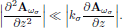
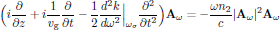
$\Big|{{\partial^2{\bf A}_{\omega_{\sigma}}}\over{\partial z^2}}\Big| \ll \Big|k_{\sigma} {{\partial{\bf A}_{\omega_{\sigma}}}\over{\partial z}}\Big|.$

These three approximations, whenever applicable, further reduce the time dependent wave equation to

$\eqalign{ \Big( \pm i{{\partial}\over{\partial z}} +i{{1}\over{v_{\rm g}}} {{\partial}\over{\partial t}} -{{1}\over{2}}{{d^2 k}\over{d\omega^2}}& \Big|_{\omega_{\sigma}}{{\partial^2}\over{\partial t^2}} \Big){\bf A}_{\omega_{\sigma}}(z,t) =-{{\mu_0\omega^2_{\sigma}}\over{2k_{\sigma}}} {\bf P}^{({\rm NL})}_{\omega_{\sigma}}({\bf r},t) \exp(\mp ik_{\sigma}z).\cr } \eqno{(4)}$ (4)

This form of the wave equation is identical to Butcher and Cotter's Eq. (7.24), with the exception that here waves propagating in positive (upper signs) as well as negative (lower signs) z-direction are considered.

7. Monochromatic light

7.1. Monochromatic optical field

$\eqalign{ {\bf E}({\bf r},t)&=\sum_{\sigma} \Re[{\bf E}_{\omega_{\sigma}}({\bf r})\exp(-i\omega_{\sigma} t)], \qquad\omega_{\sigma}\ge 0\cr {\bf E}({\bf r},\omega) &={{1}\over{2}}\sum_{\sigma} [{\bf E}_{\omega_{\sigma}}({\bf r})\delta(\omega-\omega_{\sigma}) +{\bf E}^*_{\omega_{\sigma}}({\bf r})\delta(\omega+\omega_{\sigma})]\cr }$

7.2. Polarization density induced by monochromatic optical field

${\bf P}^{(n)}({\bf r},t)=\sum_{\omega_{\sigma}\ge 0} {\rm Re}[{\bf P}^{(n)}_{\omega_{\sigma}}\exp(-i\omega_{\sigma} t)], \qquad\omega_{\sigma}=\omega_1+\omega_2+\ldots+\omega_n$

(For construction of P⁽ⁿ⁾_{ω_σ}, see notes on the Butcher and Cotter convention handed out during the third lecture.)

8. Monochromatic light - Time independent problems

For strictly monochromatic light, as for example the output light of continuous wave lasers, the temporal field envelopes are constants in time, and the wave equation (3)is reduced to

$\eqalign{ \nabla\times\nabla\times{\bf E}_{\omega_{\sigma}}({\bf r}) -k^2_{\sigma}{\bf E}_{\omega_{\sigma}}({\bf r}) =\mu_0\omega^2_{\sigma} {\bf P}^{({\rm NL})}_{\omega_{\sigma}}({\bf r}).\cr } \eqno{(5)}$ (5)

By applying the above listed approximations, one immediately finds the monochromatic, time independent form of Eq. (3) in the infinite plane wave limit and slowly varying approximation as

$\eqalign{ {{\partial}\over{\partial z}}{\bf A}_{\omega_{\sigma}} =\pm i{{\mu_0\omega^2_{\sigma}}\over{2k_{\sigma}}} {\bf P}^{({\rm NL})}_{\omega_{\sigma}} \exp(\mp ik_{\sigma}z),\cr } \eqno{(6)}$ (6)

where the upper/lower sign correspond to a wave propagating in the positive/negative z-direction. (This equation corresponds to Butcher and Cotter's Eq. (7.17).)

9. Example I: Optical Kerr-effect - Time independent case

In this example, we consider continuous wave propagation (that is to say, a time independent problem with the temporal envelope of the electrical field being constant in time) in optical Kerr-media, using light polarized in the x-direction and propagating along the positive direction of the z-axis,

${\bf E}({\bf r},t)=\Re[{\bf E}_{\omega}(z)\exp(-i\omega t)], \qquad{\bf E}_{\omega}(z)={\bf A}_{\omega}(z)\exp(ikz) ={\bf e}_x A^x_{\omega}(z)\exp(ikz),$

where, as previously, k = ωn₀/c. From material handed out during the third lecture (notes on the Butcher and Cotter convention), the nonlinear polarization density for x-polarized light is given as P^(NL)_ω = P⁽³⁾_ω, with

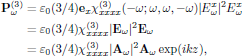
$\eqalign{ {\bf P}^{(3)}_{\omega} &=\varepsilon_0(3/4){\bf e}_x\chi^{(3)}_{xxxx} (-\omega;\omega,\omega,-\omega) |E^x_{\omega}|^2 E^x_{\omega}\cr &=\varepsilon_0(3/4)\chi^{(3)}_{xxxx} |{\bf E}_{\omega}|^2 {\bf E}_{\omega}\cr &=\varepsilon_0(3/4)\chi^{(3)}_{xxxx} |{\bf A}_{\omega}|^2 {\bf A}_{\omega}\exp(ikz),\cr }$

and the time independent wave equation for the field envelope A_ω, using Eq. (6), becomes

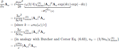
$\eqalign{ {{\partial}\over{\partial z}}{\bf A}_{\omega} &=i{{\mu_0\omega^2}\over{2k}} \underbrace{\varepsilon_0(3/4)\chi^{(3)}_{xxxx} |{\bf A}_{\omega}|^2 {\bf A}_{\omega}\exp(ikz)}_{ ={\bf P}^{({\rm NL})}_{\omega}(z)}\exp(-ikz)\cr &=i{{3\omega^2}\over{8c^2k}}\chi^{(3)}_{xxxx} |{\bf A}_{\omega}|^2 {\bf A}_{\omega}\cr &=\{{\rm since\ }k=\omega n_0(\omega)/c\}\cr &=i{{3\omega}\over{8cn_0}} \chi^{(3)}_{xxxx} |{\bf A}_{\omega}|^2 {\bf A}_{\omega}\cr &=\{{\rm in\ analogy\ with\ Butcher\ and\ Cotter\ Eq.~(6.63),\ } n_2=({{3}/{8n_0}})\chi^{(3)}_{xxxx}\}\cr &=i {{\omega n_2}\over{c}} |{\bf A}_{\omega}|^2 {\bf A}_{\omega},\cr }$

or, equivalently, in its scalar form

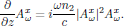
${{\partial}\over{\partial z}}A^x_{\omega} =i {{\omega n_2}\over{c}} |A^x_{\omega}|^2 A^x_{\omega}.$

If the medium of interest now is analyzed at an angular frequency far from any resonance, we may look for solutions to this equation with |A_ω| being constant (for a lossless medium). For such a case it is straightforward to integrate the final wave equation to yield the general solution

${\bf A}_{\omega}(z)= {\bf A}_{\omega}(z_0)\exp[i\omega n_2 |{\bf A}_{\omega}(z_0)|^2 z/c],$

or, again equivalently, in the scalar form (as we consider an electric field polarized along the x-axis)

$A^x_{\omega}(z)= A^x_{\omega}(z_0)\exp[i\omega n_2 |A^x_{\omega}(z_0)|^2 z/c],$

which hence gives the solution for the real-valued electric field ${\bf E}({\bf r},t)$ as

$\eqalign{ {\bf E}({\bf r},t)&=\Re[{\bf E}_{\omega}(z)\exp(-i\omega t)]\cr &=\Re\{{\bf A}_{\omega}(z)\exp[i(kz-\omega t)]\}\cr &=\Re\{{\bf A}_{\omega}(z_0) \exp[i(kz+\omega n_2 |{\bf A}_{\omega}(z_0)|^2 z/c-\omega t)]\}.\cr }$

From this solution, one immediately finds that the wave propagates with an effective propagation constant

$k+\omega n_2 |{\bf A}_{\omega}(z_0)|^2/c = (\omega/c) (n_0+ n_2 |{\bf A}_{\omega}(z_0)|^2),$

that is to say, experiencing the intensity dependent refractive index

$n_{\rm eff}=n_0+ n_2 |{\bf A}_{\omega}(z_0)|^2.$

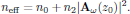
10. Example II: Optical Kerr-effect - Time dependent case

We now consider a time dependent envelope E_ω(z,t) of an optical wave propagating in the same medium and geometry as in the previous example, for which now

${\bf E}({\bf r},t)=\Re[{\bf E}_{\omega}(z,t)\exp(-i\omega t)], \qquad{\bf E}_{\omega}(z,t)={\bf A}_{\omega}(z,t)\exp(ikz) ={\bf e}_x A^x_{\omega}(z,t)\exp(ikz).$

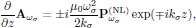
The proper wave equation to apply for this case is the time dependent wave equation (4), and since the nonlinear polarization density of the medium still is given by the optical Kerr-effect, we obtain

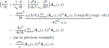
$\eqalign{ \Big( i{{\partial}\over{\partial z}} &+i{{1}\over{v_{\rm g}}} {{\partial}\over{\partial t}} -{{1}\over{2}}{{d^2 k}\over{d\omega^2}} \Big|_{\omega_{\sigma}}{{\partial^2}\over{\partial t^2}} \Big){\bf A}_{\omega}(z,t)\cr &=-{{\mu_0\omega^2}\over{2k}} \underbrace{\varepsilon_0(3/4)\chi^{(3)}_{xxxx} |{\bf A}_{\omega}(z,t)|^2 {\bf A}_{\omega}(z,t)\exp(ikz)}_{ ={\bf P}^{({\rm NL})}_{\omega}(z,t)} \exp(-ikz)\cr &=-{{3\omega^2}\over{8c^2k}} \chi^{(3)}_{xxxx} |{\bf A}_{\omega}(z,t)|^2 {\bf A}_{\omega}(z,t)\cr &=\{{\rm as\ in\ previous\ example}\}\cr &=-{{\omega n_2}\over{c}} |{\bf A}_{\omega}(z,t)|^2 {\bf A}_{\omega}(z,t).\cr }$

The resulting wave equation

is the starting point for analysis of solitons and solitary waves in optical Kerr-media. The obtained equation is the non-normalized form of the in nonlinear physics (not only nonlinear optics!) often encountered nonlinear Schrödinger equation (or NLSE, as its common acronym yields).

For a discussion on the transformation that cast the nonlinear Schrödinger equation into its normalized form, see Butcher and Cotter, page 240.

References

[1] J. D. Jackson, Classical Electrodynamics, 2nd Edn. (Wiley, New York, 1975).

[2] J. A. Stratton, Electromagnetic Theory (Mc Graw-Hill, New York, 1941).

[3] From the inverse Fourier integral identity, with the sign conventions as here used, it follows that the Fourier transform of a derivative of a function f(t) is

$\fourier[f'(t)](\omega)=-i\omega\fourier[f(t)](\omega)\qquad \Rightarrow\qquad\fourier[f''(t)](\omega) =-\omega^2\fourier[f(t)](\omega).$

[4] Notice that for isotropic media,

$$\chi^{(1)}_{\mu\alpha}(-\omega;\omega) =\chi^{(1)}_{xx}(-\omega;\omega)\delta_{\mu\alpha}$,$

which leads to the simplified form

${\bf e}_{\mu}\varepsilon_{\mu\alpha}(\omega)E_{\alpha}({\bf r},\omega) =\varepsilon(\omega){\bf E}({\bf r},\omega).$

We will here, however, continue with the general form, in order not to loose generality in discussion that is to follow.

[5] Notice that unless we apply the second approximation in the Taylor expansion of k²(ω), terms containing the squares of the derivatives will appear, which will lead to wave equations that differ from the ones given by Butcher and Cotter. In particular, this situation will arise even if one uses the suggested expansion given by Eq. (7.23) in Butcher and Cotter's book, which hence should be taken with some care if one wish to build a strict foundation for the time-dependent wave equation.

Return to previous page