Lectures on Nonlinear Optics - Lecture 6
Quantum mechanics III: Linking the microcscopic to the macroscopic
lect6.pdf [283 kB] Lecture 6 in Portable Document Format.
Contents
- Assembly of independent molecules
- First order electric susceptibility
- Second order electric susceptibility
- Overall permutation symmetry of second order susceptibility
1. Assembly of independent molecules
So far the description of the interaction between light and matter has been in a very general form, where it was assumed merely that the interaction is local, and in the electric dipolar approximation, where magnetic dipolar and electric quadrupolar interactions (as well as higher order terms) were neglected. The ensemble of molecules has so far no constraints in terms of composition or mutual interaction, and the electric dipolar operator is so far taken for the whole ensemble of molecules, rather than as the dipole operator for the individual molecules.
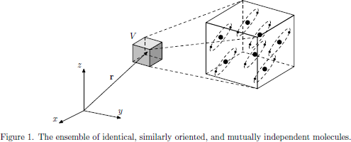
For many practical applications, however, the obtained general form is somewhat inconvenient when it comes to the numerical evaluation of the susceptibilities, since tables of wave functions, transition frequencies and their corresponding electric dipole moments etc. often are tabulated exclusively for the individual molecules themselves. Thus, we will now apply the obtained general theory to an ensemble of identical molecules, making a transition from the wave function and electric dipole operator of the whole ensemble to the wave function and electric dipole operator of the individual molecule, and find an explicit form of the electric susceptibilities in terms of the quantum mechanical matrix elements of the molecular dipole operator.
We will now apply three assumptions of the ensemble of molecules, which introduce a significant simplification to the task of expressing the susceptibilities and macroscopic polarization density in terms of the individual molecular properties:
- The molecules of the ensemble are all identical.
- The molecules of the ensemble are mutually non-interacting.
- The molecules of the ensemble are identically oriented.
From a wave functional approach, it is straightforward to make the transition from the description of the ensemble down to the molecular level in a strict quantum mechanical perspective (as shown in Butcher and Cotters book). However, from a practical engineering point of view, the results are quite intuitively derived if we make the following observations, which immediately follow from the assumptions listed above:
- The positions of the individual molecules does not affect the electric dipole moment of the whole ensemble in V, if we neglect the mutual interaction between the molecules. (This holds only if the molecules are neutrally charged, since they otherwise could build up a total electric dipole moment of the ensemble.)
- Since the mutual interaction between the molecules is
neglected, we may just as well consider the individual molecules as
constituting a set of "sub-ensembles" of the general ensemble picture.
In this picture, all quantum mechanical expectation values, involved
commutators, matrix elements, etc., should be considered for each
subensemble instead, and the macroscopic polarization density will
in this case become

Assuming there are M mutually non-interacting and similarly oriented molecules in the volume V, the macroscopic polarization density of the medium can be written as
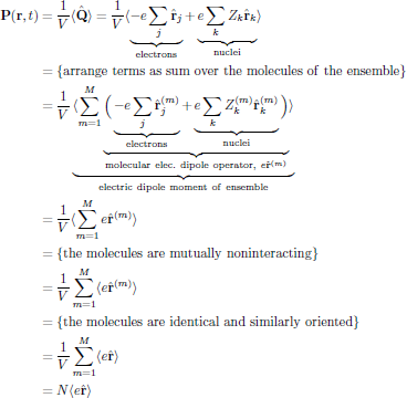
where N = M/V is the number of molecules per unit volume, and
![$$
\langle e\hat{\bf r}\rangle=\Tr[\hat{\varrho}(t) e\hat{\bf r}]
$$](/research/lectures/lect6/web/images_80proc/lect6_eq_disp_003.png)
is the expectation value of the mono-molecular electric dipole
operator, with
 (that is to say,
 with a
"kink" [1] to indicate the difference to the density
operator of the general ensemble) is the molecular density operator.
Notice that the form
with a
"kink" [1] to indicate the difference to the density
operator of the general ensemble) is the molecular density operator.
Notice that the form
 is identical to the previous form for the general ensemble, though with
the factor 1/V replaced by N = M/V,
and with the electric dipole operator
is identical to the previous form for the general ensemble, though with
the factor 1/V replaced by N = M/V,
and with the electric dipole operator
 of the ensemble replaced by the
molecular dipole moment operator
of the ensemble replaced by the
molecular dipole moment operator
 .
.
When making this transition, the condition that the molecules are mutually independent is simply a statement that we locally assume the superposition principle of the properties of the molecules (wave functions, electric dipole moments, etc.) to hold.
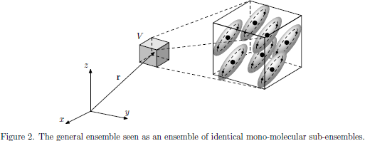
Going in the limit of non-interacting molecules, we may picture the situation as in Fig. 2, with each molecule defining a sub-ensemble, which we are free to choose as our "small volume" of charged particles. As long as we do not make any claim to determine the exact individual positions of the charged particles together with their respective momentum (or any other pair of canonical variables which would violate the Heisenberg uncertainty relation), this is a perfectly valid picture, which provides the statistical expectation values of any observable property of the medium as $M/V$ times the average statistical molecular observations.
The previously described operators of a general ensemble of charged particles should in this case be replaced by their corresponding mono-molecular equivalents, as listed in the following table.
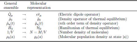
Whenever an operator is expressed in the interaction picture, we should keep in mind that the corresponding time development operators $\hat{U}_0(t)$, which originally were expressed in terms of the thermal equilibrium Hamiltonian $\hat{H}_0$ of the ensemble, now should be expressed in terms of the mono-molecular thermal equilibrium Hamiltonian $\hat{\cal H}_0$.
The matrix elements of the mono-molecular electric dipole operator, taken in the interaction picture, become
![$$
\eqalign{
\langle a|e\hat{r}_{\alpha}(t)|b\rangle
&=\langle a|\hat{U}_0(-t)e\hat{r}_{\alpha}\hat{U}_0(t)|b\rangle\cr
&=\{{\rm the\ closure\ principle,\ B.\&C.\ Eq.~(3.11),\ }
[\hat{O}\hat{O}']_{ab}=\sum_k O_{ak}O_{kb}\}\cr
&=\sum_k\sum_l
\langle a|\hat{U}_0(-t)|k\rangle
\langle k|e\hat{r}_{\alpha}|l\rangle
\langle l|\hat{U}_0(t)|b\rangle\cr
&=\{{\rm energy\ representation,\ B.\&C.\ Eq.~(4.54),\ }
[\hat{U}_0(t)]_{ab}=\exp(-i{\Bbb E}_a t/\hbar)\delta_{ab}\}\cr
&=\sum_k\sum_l
\exp(-i{\Bbb E}_a (-t)/\hbar)\delta_{ak}
\langle k|e\hat{r}_{\alpha}|l\rangle
\exp(-i{\Bbb E}_l t/\hbar)\delta_{lb}\cr
&=\langle a|e\hat{r}_{\alpha}|b\rangle\exp[
i\underbrace{({\Bbb E}_a-{\Bbb E}_b)t/\hbar}_{\equiv\Omega_{ab}t}]\cr
&=\langle a|e\hat{r}_{\alpha}|b\rangle\exp(i\Omega_{ab}t),\cr
}\eqno{(3)}
$$](/research/lectures/lect6/web/images_80proc/lect6_eq_disp_005.png) (1)
(1)where

is the molecular transition
frequency between the molecular states
 and
and
 .
We may thus, at least in some sense, interpret the interaction picture
for the matrix elements of the molecular operators as an out-separation
of the naturally occurring transition frequencies associated with a change
from state
and
of the molecule.
.
We may thus, at least in some sense, interpret the interaction picture
for the matrix elements of the molecular operators as an out-separation
of the naturally occurring transition frequencies associated with a change
from state
and
of the molecule.
2. First order electric susceptibility
From the general form of the first order (linear) electric susceptibility, as derived in the previous lecture, one obtains
![$$
\eqalign{
\chi^{(1)}_{\mu\alpha}(-\omega;\omega)
&=-{{N}\over{\varepsilon_0 i\hbar}}\int^0_{-\infty}
\Tr\{\hat{\varrho}_0[e\hat{r}_{\mu},e\hat{r}_{\alpha}(\tau)]\}
\exp(-i\omega\tau)\,d\tau\cr
&=-{{N e^2}\over{\varepsilon_0 i\hbar}}\int^0_{-\infty}
\sum_a\langle a|\hat{\varrho}_0(\hat{r}_{\mu}\hat{r}_{\alpha}(\tau)
-\hat{r}_{\alpha}(\tau)\hat{r}_{\mu})|a\rangle
\exp(-i\omega\tau)\,d\tau\cr
&=\{{\rm the\ closure\ principle}\}\cr
&=-{{N e^2}\over{\varepsilon_0 i\hbar}}\int^0_{-\infty}
\sum_a\sum_k
\langle a|\hat{\varrho}_0|k\rangle
\langle k|\hat{r}_{\mu}\hat{r}_{\alpha}(\tau)
-\hat{r}_{\alpha}(\tau)\hat{r}_{\mu}|a\rangle
\exp(-i\omega\tau)\,d\tau\cr
&=\{{\rm use\ that\ }
\langle a|\hat{\varrho}_0|k\rangle=\varrho_0(a)\delta_{ak}\}\cr
&=-{{N e^2}\over{\varepsilon_0 i\hbar}}\int^0_{-\infty}
\sum_a\varrho_0(a)
\big[\langle a|\hat{r}_{\mu}\hat{r}_{\alpha}(\tau)|a\rangle
-\langle a|\hat{r}_{\alpha}(\tau)\hat{r}_{\mu}|a\rangle\big]
\exp(-i\omega\tau)\,d\tau\cr
&=\{{\rm the\ closure\ principle\ again}\}\cr
&=-{{N e^2}\over{\varepsilon_0 i\hbar}}\int^0_{-\infty}
\sum_a\varrho_0(a)\sum_b
\big[\langle a|\hat{r}_{\mu}|b\rangle
\langle b|\hat{r}_{\alpha}(\tau)|a\rangle
-\langle a|\hat{r}_{\alpha}(\tau)|b\rangle
\langle b|\hat{r}_{\mu}|a\rangle\big]
\exp(-i\omega\tau)\,d\tau\cr
&=\{{\rm Use\ results\ of\ Eq.~(3)\ and\ shorthand\ notation\ }
\langle a|\hat{r}_{\alpha}|b\rangle=r^{\alpha}_{ab}\}\cr
&=-{{N e^2}\over{\varepsilon_0 i\hbar}}
\sum_a\varrho_0(a)\sum_b\int^0_{-\infty}
\big[r^{\mu}_{ab}r^{\alpha}_{ba}\exp(i\Omega_{ba}\tau)
-r^{\alpha}_{ab}r^{\mu}_{ba}\exp(-i\Omega_{ba}\tau)\big]
\exp(-i\omega\tau)\,d\tau\cr
&=\{{\rm evaluate\ integral\ }
\int^0_{-\infty}\exp(iC\tau)\,d\tau\to 1/(iC)\}\cr
&=-{{N e^2}\over{\varepsilon_0 i\hbar}}
\sum_a\varrho_0(a)\sum_b
\Big[{{r^{\mu}_{ab}r^{\alpha}_{ba}}\over{i(\Omega_{ba}-\omega)}}
-{{r^{\alpha}_{ab}r^{\mu}_{ba}}\over{-i(\Omega_{ba}+\omega)}}\Big]\cr
&={{N e^2}\over{\varepsilon_0\hbar}}
\sum_a\varrho_0(a)\sum_b
\Big({{r^{\mu}_{ab}r^{\alpha}_{ba}}\over{\Omega_{ba}-\omega}}
+{{r^{\alpha}_{ab}r^{\mu}_{ba}}\over{\Omega_{ba}+\omega}}\Big).\cr
}
$$](/research/lectures/lect6/web/images_80proc/lect6_eq_disp_007.png)
This result, which was derived entirely under the assumption that all resonances of the medium are located far away from the angular frequency of the light, possesses a new type of symmetry, which can be seen if we make the interchange

which by using the above result for the linear susceptibility gives
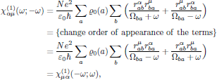
which is a signature of the overall permutation symmetry that applies to nonresonant interactions. With this result, the reason for the peculiar notation "(-ω ; ω)" should be all clear, namely that it serves as an explicit way of notation of the overall permutation symmetry, whenever it applies.
It should be noticed that while intrinsic permutation symmetry is a general property that solely applies to nonlinear optical interactions, the overall permutation symmetry applies to linear interactions as well.
3. Second order electric susceptibility
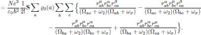
In similar to the linear electric susceptibility, starting from the general form of the second order (quadratic) electric susceptibility, one obtains
![$$
\eqalign{
\chi^{(2)}_{\mu\alpha\beta}&(-\omega_{\sigma};\omega_1,\omega_2)\cr
&={{N e^3}\over{\varepsilon_0 (i\hbar)^2}}
{{1}\over{2!}}{\bf S}
\int^0_{-\infty}\int^{\tau_1}_{-\infty}
\Tr\{\hat{\varrho}_0[[\hat{r}_{\mu},\hat{r}_{\alpha}(\tau_1)],
\hat{r}_{\beta}(\tau_2)]\}
\exp[-i(\omega_1\tau_1+\omega_2\tau_2)]
\,d\tau_2\,d\tau_1\cr
&={{N e^3}\over{\varepsilon_0 (i\hbar)^2}}
{{1}\over{2!}}{\bf S}
\int^0_{-\infty}\int^{\tau_1}_{-\infty}
\sum_a\langle a|\hat{\varrho}_0[
\underbrace{[\hat{r}_{\mu},\hat{r}_{\alpha}(\tau_1)]}_{
\hat{r}_{\mu}\hat{r}_{\alpha}(\tau_1)
-\hat{r}_{\alpha}(\tau_1)\hat{r}_{\mu}},
\hat{r}_{\beta}(\tau_2)]|a\rangle
\exp[-i(\omega_1\tau_1+\omega_2\tau_2)]
\,d\tau_2\,d\tau_1\cr
&=\{{\rm expand\ the\ commutator}\}\cr
&={{N e^3}\over{\varepsilon_0 (i\hbar)^2}}
{{1}\over{2!}}{\bf S}
\int^0_{-\infty}\int^{\tau_1}_{-\infty}
\sum_a\Big(
\langle a|\hat{\varrho}_0\hat{r}_{\mu}
\hat{r}_{\alpha}(\tau_1)\hat{r}_{\beta}(\tau_2)|a\rangle
-\langle a|\hat{\varrho}_0\hat{r}_{\alpha}(\tau_1)
\hat{r}_{\mu}\hat{r}_{\beta}(\tau_2)|a\rangle
\cr&\qquad\qquad
-\langle a|\hat{\varrho}_0\hat{r}_{\beta}(\tau_2)
\hat{r}_{\mu}\hat{r}_{\alpha}(\tau_1)|a\rangle
+\langle a|\hat{\varrho}_0\hat{r}_{\beta}(\tau_2)
\hat{r}_{\alpha}(\tau_1)\hat{r}_{\mu}|a\rangle
\Big)\exp[-i(\omega_1\tau_1+\omega_2\tau_2)]
\,d\tau_2\,d\tau_1\cr
&=\{{\rm apply\ the\ closure\ principle\ and\ Eq.~(3)}\}\cr
&={{N e^3}\over{\varepsilon_0 (i\hbar)^2}}
{{1}\over{2!}}{\bf S}
\int^0_{-\infty}\int^{\tau_1}_{-\infty}
\sum_a\sum_k\sum_b\sum_c\Big(
\langle a|\hat{\varrho}_0|k\rangle
\langle k|\hat{r}_{\mu}|b\rangle
\langle b|\hat{r}_{\alpha}(\tau_1)|b\rangle
\langle c|\hat{r}_{\beta}(\tau_2)|a\rangle
\cr&\qquad\qquad\qquad\qquad
-\langle a|\hat{\varrho}_0|k\rangle
\langle k|\hat{r}_{\alpha}(\tau_1)|b\rangle
\langle b|\hat{r}_{\mu}|c\rangle
\langle c|\hat{r}_{\beta}(\tau_2)|a\rangle
\cr&\qquad\qquad\qquad\qquad
-\langle a|\hat{\varrho}_0|k\rangle
\langle k|\hat{r}_{\beta}(\tau_2)|b\rangle
\langle b|\hat{r}_{\mu}|c\rangle
\langle c|\hat{r}_{\alpha}(\tau_1)|a\rangle
\cr&\qquad\qquad\qquad\qquad
+\langle a|\hat{\varrho}_0|k\rangle
\langle k|\hat{r}_{\beta}(\tau_2)|b\rangle
\langle b|\hat{r}_{\alpha}(\tau_1)|c\rangle
\langle c|\hat{r}_{\mu}|a\rangle
\Big)\exp[-i(\omega_1\tau_1+\omega_2\tau_2)]
\,d\tau_2\,d\tau_1\cr
&=\{{\rm use\ that\ }
\langle a|\hat{\varrho}_0|k\rangle=\varrho_0(a)\delta_{ak}
{\rm\ and\ apply\ Eq.~(3)}\}\cr
&={{N e^3}\over{\varepsilon_0 (i\hbar)^2}}
{{1}\over{2!}}{\bf S}
\sum_a\varrho_0(a)\sum_b\sum_c
\int^0_{-\infty}\int^{\tau_1}_{-\infty}\Big\{
r^{\mu}_{ab} r^{\alpha}_{bc} r^{\beta}_{ca}
\exp[i(\Omega_{bc}\tau_1+\Omega_{ca}\tau_2)]
\cr&\qquad\qquad\qquad\qquad
-r^{\alpha}_{ab} r^{\mu}_{bc} r^{\beta}_{ca}
\exp[i(\Omega_{ab}\tau_1+\Omega_{ca}\tau_2)]
% \cr&\qquad\qquad\qquad\qquad
-r^{\beta}_{ab} r^{\mu}_{bc} r^{\alpha}_{ca}
\exp[i(\Omega_{ca}\tau_1+\Omega_{ab}\tau_2)]
\cr&\qquad\qquad\qquad\qquad
+r^{\beta}_{ab} r^{\alpha}_{bc} r^{\mu}_{ca}
\exp[i(\Omega_{bc}\tau_1+\Omega_{ab}\tau_2)]
\Big\}\exp[-i(\omega_1\tau_1+\omega_2\tau_2)]
\,d\tau_2\,d\tau_1\cr
&={{N e^3}\over{\varepsilon_0 (i\hbar)^2}}
{{1}\over{2!}}{\bf S}
\sum_a\varrho_0(a)\sum_b\sum_c
\int^0_{-\infty}\Big\{
{{r^{\mu}_{ab} r^{\alpha}_{bc} r^{\beta}_{ca}}
\over{i(\Omega_{ca}-\omega_2)}}
\exp[i\underbrace{(\Omega_{bc}+\Omega_{ca})}_{=\Omega_{ba}}\tau_1]
\cr&\qquad\qquad\qquad\qquad
-{{r^{\alpha}_{ab} r^{\mu}_{bc} r^{\beta}_{ca}}
\over{i(\Omega_{ca}-\omega_2)}}
\exp[i\underbrace{(\Omega_{ab}+\Omega_{ca})}_{=\Omega_{cb}}\tau_1]
% \cr&\qquad\qquad\qquad\qquad
-{{r^{\beta}_{ab} r^{\mu}_{bc} r^{\alpha}_{ca}}
\over{i(\Omega_{ab}-\omega_2)}}
\exp[i\underbrace{(\Omega_{ca}+\Omega_{ab})}_{=\Omega_{cb}}\tau_1)]
\cr&\qquad\qquad\qquad\qquad
+{{r^{\beta}_{ab} r^{\alpha}_{bc} r^{\mu}_{ca}}
\over{i(\Omega_{ab}-\omega_2)}}
\exp[i\underbrace{(\Omega_{bc}+\Omega_{ab})}_{=-\Omega_{ca}}\tau_1]
\Big\}\exp[-i\underbrace{(\omega_1+\omega_2)}_{=\omega_{\sigma}}\tau_1]
\,d\tau_1\cr
&={{N e^3}\over{\varepsilon_0 (i\hbar)^2}}
{{1}\over{2!}}{\bf S}
\sum_a\varrho_0(a)\sum_b\sum_c
\Big\{
-{{r^{\mu}_{ab} r^{\alpha}_{bc} r^{\beta}_{ca}}
\over{(\Omega_{ca}-\omega_2)(\Omega_{ba}-\omega_{\sigma})}}
+{{r^{\alpha}_{ab} r^{\mu}_{bc} r^{\beta}_{ca}}
\over{(\Omega_{ca}-\omega_2)(\Omega_{cb}-\omega_{\sigma})}}
\cr&\qquad\qquad\qquad\qquad
+{{r^{\beta}_{ab} r^{\mu}_{bc} r^{\alpha}_{ca}}
\over{(\Omega_{ab}-\omega_2)(\Omega_{cb}-\omega_{\sigma})}}
-{{r^{\beta}_{ab} r^{\alpha}_{bc} r^{\mu}_{ca}}
\over{(\Omega_{ab}-\omega_2)(-\Omega_{ca}-\omega_{\sigma})}}
\Big\}\cr
&\hskip 90mm\ldots{\it continued\ on\ next\ page}\ldots\cr
}
$$](/research/lectures/lect6/web/images_80proc/lect6_eq_disp_010.png)
4. Overall permutation symmetry of second order susceptibility
Now it is easily seen that if we, for example, interchange
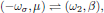
one obtains
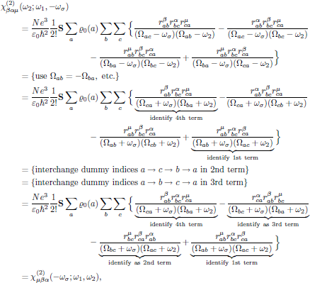
that is to say, the second order susceptibility is left invariant under any of the (2 + 1)! = 6 possible pairwise permutations of (-ωσ,μ), (ω1,α), and (ω2,β); this is the overall permutation symmetry for the second order susceptibility, and applies whenever the interaction is moved far away from any resonance.
We recapitulate that when deriving the form of the nonlinear susceptibilities that lead to intrinsic permutation symmetry, either in terms of polarization response functions in time domain or in terms of a mechanical spring model, nothing actually had to be stated regarding the nature of interaction. This is rather different from what we just obtained for the overall permutation symmetry, as being a signature of a nonresonant interaction between the light and matter, and this symmetry cannot (in contrary to the intrinsic permutation symmetry) be expressed unless the origin of interaction is considered. (It should though be noticed that the derivation of the susceptibilities still may be performed within a mechanical spring model, as long as the resonance frequencies of the oscillator are removed far from the angular frequencies of the present light.)
References
[1] kink n. 1. a sharp twist or bend in a wire, rope, hair, etc. [Collins Concise Dictionary, Harper-Collins (1995)].