Lectures on Nonlinear Optics - Lecture 3
Quasi-monochromatic fields and the degeneracy factor in nonlinear optics
lect3.pdf [283 kB] Lecture 3 in Portable Document Format.
Contents
- Susceptibility tensors in the frequency domain
- First order susceptibility tensor
- Second order susceptibility tensor
- Higher order susceptibility tensors
- Monochromatic fields
- Convention for description of nonlinear optical polarization
1. Susceptibility tensors in the frequency domain
The susceptibility tensors in the frequency domain arise when the electric field Eα(t) of the light is expressed in terms of its Fourier transform Eα(ω), by means of the Fourier integral identity
,\eqno{(1')}
$$](/research/lectures/lect3/web/images_80proc/lect3_eq_disp_001.png) (1)
(1).\eqno{(1'')}
$$](/research/lectures/lect3/web/images_80proc/lect3_eq_disp_002.png) (2)
(2)This convention of inclusion of the factor of 2π, as well as the sign convention, is commonly used in quantum mechanics; however, it should be emphasized that this convention is not a commonly adopted standard in optics, neither in linear nor in nonlinear optical regimes.
The sign convention here used leads to wave solutions of the form f(kz-ωt) for monochromatic waves propagating in the positive z-direction, which might be somewhat more intuitive than the alternative form f(ωt-kz), which is obtained if one instead apply the alternative sign convention.
The convention for the inclusion of 2π in the Fourier transform in Eq. (2) is here convenient for description of electromagnetic wave propagation in the frequency domain (going from the time domain description, in terms of the polarization response functions, to the frequency domain, in terms of the linear and nonlinear susceptibilities), since it enables us to omit any multiple of 2π of the Fourier transformed fields.
2. First order susceptibility tensor
By inserting Eq. (1) into the previously obtained relation for the first order, linear polarization density (See the expressions for the first order, second order, and n:th order polarization densities as obtained in lecture two), one obtains
![$$
\eqalign{
P^{(1)}_{\mu}({\bf r},t)
&=\varepsilon_0\int^{\infty}_{-\infty}
R^{(1)}_{\mu\alpha}(\tau) E_{\alpha}({\bf r},t-\tau)\,d\tau,\cr
&=\{{\rm express}\ E_{\alpha}({\bf r},t-\tau)
\ {\rm in\ frequency\ domain}\}\cr
&=\varepsilon_0\int^{\infty}_{-\infty}
R^{(1)}_{\mu\alpha}(\tau)\int^{\infty}_{-\infty}
E_{\alpha}({\bf r},\omega)
\exp[-i\omega(t-\tau)]\,d\omega\,d\tau,\cr
&=\{{\rm change\ order\ of\ integration}\}\cr
&=\varepsilon_0\int^{\infty}_{-\infty}\int^{\infty}_{-\infty}
R^{(1)}_{\mu\alpha}(\tau) E_{\alpha}({\bf r},\omega)
\exp(i\omega\tau)\,d\tau\,\exp(-i\omega t)\,d\omega,\cr
&=\varepsilon_0\int^{\infty}_{-\infty}
\chi^{(1)}_{\mu\alpha}(-\omega;\omega)
E_{\alpha}({\bf r},\omega)
\exp(-i\omega t)\,d\omega,\cr
}\eqno{(2)}
$$](/research/lectures/lect3/web/images_80proc/lect3_eq_disp_003.png) (3)
(3)where the linear electric dipolar susceptibility,
(4)was introduced. In this expression for the susceptibility, the frequency argument is ωσ = ω, and the reasons for the somewhat peculiar notation of arguments of the susceptibility will be explained later on in the context of nonlinear susceptibilities.
3. Second order susceptibility tensor
In similar to the linear susceptibility tensor, by inserting Eq. (1) into the previously obtained relation for the second order, quadratic polarization density, one obtains
![$$
\eqalign{
P^{(2)}_{\mu}({\bf r},t)
&=\varepsilon_0
\int^{\infty}_{-\infty}\int^{\infty}_{-\infty}
\int^{\infty}_{-\infty}\int^{\infty}_{-\infty}
R^{(2)}_{\mu\alpha\beta}(\tau_1,\tau_2)
E_{\alpha}({\bf r},\omega_1) E_{\beta}({\bf r},\omega_2)
\cr&\qquad\qquad\qquad\times
\exp[-i(\omega_1(t-\tau_1)+\omega_2(t-\tau_2))]
\,d\tau_1\,d\tau_2
\,d\omega_1\,d\omega_2\cr
&=\varepsilon_0
\int^{\infty}_{-\infty}\int^{\infty}_{-\infty}
\chi^{(2)}_{\mu\alpha\beta}(-\omega_{\sigma};\omega_1,\omega_2)
E_{\alpha}({\bf r},\omega_1) E_{\beta}({\bf r},\omega_2)
\exp[-i\underbrace{(\omega_1+\omega_2)}_{\equiv\omega_{\sigma}}t]
\,d\omega_1\,d\omega_2\cr
}\eqno{(4)}
$$](/research/lectures/lect3/web/images_80proc/lect3_eq_disp_005.png) (5)
(5)where the quadratic electric dipolar susceptibility,
![$$
\chi^{(2)}_{\mu\alpha\beta}(-\omega_{\sigma};\omega_1,\omega_2)
=\int^{\infty}_{-\infty}\int^{\infty}_{-\infty}
R^{(2)}_{\mu\alpha\beta}(\tau_1,\tau_2)
\exp[i(\omega_1\tau_1+\omega_2\tau_2)]\,d\tau_1\,d\tau_2,\eqno{(5)}
$$](/research/lectures/lect3/web/images_80proc/lect3_eq_disp_006.png) (6)
(6)was introduced. In this expression for the susceptibility, ωσ = ω1+ω2 denotes the resulting angular frequency of the induced polarization density (and from the oscillating polarization density, this is also the angular frequency of the resulting electric field of the induced light wave). The reason for the notation of arguments should now be somewhat more clear: the first angular frequency argument of the susceptibility tensor is simply the sum of all driving angular frequencies of the optical field.
The intrinsic permutation symmetry of R(2)μαβ(τ1,τ2), the second order polarization response function, carries over to the second order susceptibility tensor as well, in the sense that
 (7)
(7)that is to say, the second order susceptibility is invariant under any of the 2! = 2 pairwise permutations of (α,ω1) and (β,ω2).
4. Higher order susceptibility tensors
In similar to the linear and quadratic susceptibility tensors, by inserting Eq. (1) into the previously obtained relation for the n:th order polarization density, one obtains
![$$
\eqalign{
P^{(n)}_{\mu}({\bf r},t)
&=\varepsilon_0
\int^{\infty}_{-\infty}\cdots\int^{\infty}_{-\infty}
\chi^{(n)}_{\mu\alpha_1\cdots\alpha_n}
(-\omega_{\sigma};\omega_1,\ldots,\omega_n)
E_{\alpha_1}({\bf r},\omega_1)\cdots
E_{\alpha_n}({\bf r},\omega_n)
\cr&\qquad\qquad\qquad\times
\exp[-i\underbrace{(\omega_1+\ldots+\omega_n)}_{
\equiv\omega_{\sigma}}t]
\,d\omega_1\,\cdots\,d\omega_n,\cr
}\eqno{(6)}
$$](/research/lectures/lect3/web/images_80proc/lect3_eq_disp_008.png) (8)
(8)where the n:th order electric dipolar susceptibility,
![$$
\chi^{(n)}_{\mu\alpha_1\cdots\alpha_n}
(-\omega_{\sigma};\omega_1,\ldots,\omega_n)
=\int^{\infty}_{-\infty}\cdots\int^{\infty}_{-\infty}
R^{(n)}_{\mu\alpha_1\cdots\alpha_n}(\tau_1,\ldots,\tau_n)
\exp[i(\omega_1\tau_1+\ldots+\omega_n\tau_n)]\,d\tau_1\,\cdots\,d\tau_n,
\eqno{(7)}
$$](/research/lectures/lect3/web/images_80proc/lect3_eq_disp_009.png) (9)
(9)was introduced, and where, as previously,

The intrinsic permutation symmetry of R(n)μα1…αn(τ1, … , τn), the n:th order polarization response function, also in this general case carries over to the n:th order susceptibility tensor as well, in the sense that
is invariant under any of the n! pairwise permutations of (α1,ω1), (α2,ω2), …, (αn,ωn).
5. Monochromatic_fields
It should at this stage be emphasized that even though the electric field via the Fourier integral identity described by Eqs. (1) and (2) can be seen as a superposition of infinitely many infinitesimally narrow band monochromatic components, the superposition principle of linear optics, which states that the wave equation may be independently solved for each frequency component of the light, generally does not hold in nonlinear optics.
For monochromatic light, the electric field can be written as a superposition of a set of distinct terms in time domain as
![$$
{\bf E}({\bf r},t)=\sum_k \Re[{\bf E}_{\omega_k}\exp(-i\omega_k t)],
$$](/research/lectures/lect3/web/images_80proc/lect3_eq_disp_012.png)
with the convention that the involved angular frequencies all are taken as positive, that is to say with ωk ≥ 0, and the electric field in the frequency domain simply becomes a superposition of delta peaks in the spectrum,
![$$
\eqalign{
{\bf E}({\bf r},\omega)
&={{1}\over{2\pi}}\int^{\infty}_{-\infty}{\bf E}({\bf r},\tau)
\exp(i\omega\tau)\,d\tau\cr
&=\{{\rm express\ as\ monochromatic\ field}\}\cr
&={{1}\over{2\pi}}\sum_k \int^{\infty}_{-\infty}
\Re[{\bf E}_{\omega_k}\exp(-i\omega_k \tau)]
\exp(i\omega\tau)\,d\tau\cr
&=\{{\rm by\ definition}\}\cr
&={{1}\over{4\pi}}\sum_k \int^{\infty}_{-\infty}
[{\bf E}_{\omega_k}\exp(i(\omega-\omega_k)\tau)
+{\bf E}^*_{\omega_k}\exp(i(\omega+\omega_k)\tau)]\,d\tau\cr
&={{1}\over{2}}\sum_k \bigg[
{\bf E}_{\omega_k}\underbrace{{{1}\over{2\pi}}\int^{\infty}_{-\infty}
\exp(i(\omega-\omega_k)\tau)\,d\tau}_{
\equiv\delta(\omega-\omega_k)}
+{\bf E}^*_{\omega_k}
\underbrace{{{1}\over{2\pi}}\int^{\infty}_{-\infty}
\exp(i(\omega+\omega_k)\tau)\,d\tau}_{
\equiv\delta(\omega+\omega_k)}\bigg]\cr
&=\{{\rm definition\ of\ the\ delta\ function}\}\cr
&={{1}\over{2}}\sum_k [{\bf E}_{\omega_k}\delta(\omega-\omega_k)
+{\bf E}^*_{\omega_k}\delta(\omega+\omega_k)].\cr
}
$$](/research/lectures/lect3/web/images_80proc/lect3_eq_disp_013.png)
By inserting this form of the electric field (taken in the frequency domain) into the polarization density, one obtains the polarization density in the monochromatic form
![$$
{\bf P}^{(n)}({\bf r},t)=\sum_{\omega_{\sigma}\ge 0}
\Re[{\bf P}^{(n)}_{\omega_{\sigma}}\exp(-i\omega_{\sigma} t)],
$$](/research/lectures/lect3/web/images_80proc/lect3_eq_disp_014.png)
with complex-valued Cartesian components at angular frequency ωσ given as
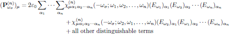 (10)
(10)where, as previously,
In the right hand side of Eq. (10), the summation is performed over all distinguishble terms, that is to say over all the possible combinations of ω1,ω2,…, ωn that give rise to the particular sum frequency ωσ. Within this respect, a certain frequency and its negative counterpart are to be considered as distinct frequencies when appearing in the set. In general, there are several possible combinations that give rise to a certain ωσ; for example (ω,ω,-ω), (ω,-ω,ω), and (-ω,ω,ω) form the set of distinct combinations of optical frequencies that give rise to optical Kerr-effect (a field dependent contribution to the polarization density at ωσ = ω+ω-ω = ω; more about this later on in this lecture).
A general conclusion of the form of Eq. (10), keeping the intrinsic permutation symmetry in mind, is that only one term needs to be written, and the number of times this term appears in the expression for the polarization density should consequently be equal to the number of distinguishable combinations of ω1,ω2,…, ωn.
6. Convention for description of nonlinear optical polarization
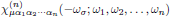
As a "recipe" in theoretical nonlinear optics, Butcher and Cotter provide a very useful convention which is well worth to hold on to. (This convention is also summarized in a separate summary of the Butcher and Cotter convention of nonlinear optical susceptibilities) For a superposition of monochromatic waves, and by invoking the general property of the intrinsic permutation symmetry, the monochromatic form of the n:th order polarization density can be written as
 (11)
(11)The first summations in Eq. (11), over α1, …, αn, is simply an explicit way of stating that the Einstein convention of summation over repeated indices holds. The summation sign over angular frequencies, Σω, however, serves as a reminder that the expression that follows is to be summed over all distinct sets of ω1, …, ωn. Because of the intrinsic permutation symmetry, the frequency arguments appearing in Eq. (11) may be written in arbitrary order.
By "all distinct sets of ω1, … , ωn", we here mean that the summation is to be performed, as for example in the case of optical Kerr-effect, over the single set of nonlinear susceptibilities that contribute to a certain angular frequency as (-ω;ω,ω,-ω) or (-ω;ω,-ω,ω) or (-ω;-ω,ω,ω). In this example, each of the combinations are considered as distinct, and it is left as an arbitary choice which one of these sets that are most convenient to use (this is simply a matter of choosing notation, and does not by any means change the description of the interaction).
In Eq. (11), the degeneracy factor K is formally described as
 (12)
(12)where
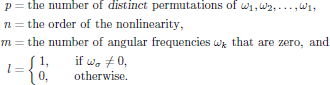
In other words, $m$ is the number of DC electric fields present, and $l=0$ if the nonlinearity we are analyzing gives a static, DC, polarization density, such as in the previously (in the spring model) described case of optical rectification in the presence of second harmonic fields (SHG).
A list of frequently encountered nonlinear phenomena in nonlinear optics, including the degeneracy factors as conforming to the above convention, is given in Butcher and Cotters book, Table 2.1, on page 26.
6.1. Note on the complex representation of the optical field
Since the observable electric field of the light, in Butcher and Cotters notation taken as
![$$
{\bf E}({\bf r},t)={{1}\over{2}}\sum_{\omega_k\ge 0}
[{\bf E}_{\omega_k}\exp(-i\omega_k t)+{\bf E}^*_{\omega_k}\exp(i\omega_k t)],
$$](/research/lectures/lect3/web/images_80proc/lect3_eq_disp_019.png)
is a real-valued quantity, it follows that negative frequencies in the complex notation should be interpreted as the complex conjugate of the respective field component, or
6.2. Example: Optical Kerr-effect
Assume a monochromatic optical wave (containing forward and/or backward propagating components) polarized in the xy-plane,
![$$
{\bf E}(z,t)=\Re[{\bf E}_{\omega}(z)\exp(-i\omega_t)]\in{\Bbb R}^3,
$$](/research/lectures/lect3/web/images_80proc/lect3_eq_disp_021.png)
with all spatial variation of the field contained in the complex-valued field envelope

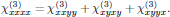
Optical Kerr-effect is in isotropic media described by the third order susceptibility

with nonzero components of interest for the xy-polarized beam given as

with (see, for example, Appendix 3.3 of Butcher and Cotter)
Since
- the number of distinct permutations of the frequency arguments (ω,ω,-ω) is p = 3,
- the order of the nonlinearity is n = 3,
- no angular frequencies of the electric field are zero (m = 0), and, finally,
- the angular frequency of the induced polarization density is non-zero (l = 1),
the degeneracy factor K(-ω;ω,ω,-ω) is calculated as

From this set of nonzero susceptibilities, and using the calculated value of the degeneracy factor in the convention of Butcher and Cotter, we hence have the third order electric polarization density at ωσ = ω given as
![${\bf P}^{(n)}({\bf r},t)=\Re[{\bf P}^{(n)}_{\omega}\exp(-i\omega t)]$](/research/lectures/lect3/web/images_80proc/lect3_eq_disp_027.png)
with
![$$
\eqalign{
{\bf P}^{(3)}_{\omega}
&=\sum_{\mu}{\bf e}_{\mu}(P^{(3)}_{\omega})_{\mu}\cr
&=\{{\rm Using\ the\ convention\ of\ Butcher\ and\ Cotter}\}\cr
&=\sum_{\mu}{\bf e}_{\mu}
\bigg[\varepsilon_0{{3}\over{4}}\sum_{\alpha}\sum_{\beta}\sum_{\gamma}
\chi^{(3)}_{\mu\alpha\beta\gamma}(-\omega;\omega,\omega,-\omega)
(E_{\omega})_{\alpha}(E_{\omega})_{\beta}(E_{-\omega})_{\gamma}\bigg]\cr
&=\{{\rm Evaluate\ the\ sums\ over\ } (x,y,z)
{\rm\ for\ field\ polarized\ in\ the\ }xy{\rm\ plane}\}\cr
&=\varepsilon_0{{3}\over{4}}\{
{\bf e}_x[
\chi^{(3)}_{xxxx} E^x_{\omega} E^x_{\omega} E^x_{-\omega}
+\chi^{(3)}_{xyyx} E^y_{\omega} E^y_{\omega} E^x_{-\omega}
+\chi^{(3)}_{xyxy} E^y_{\omega} E^x_{\omega} E^y_{-\omega}
+\chi^{(3)}_{xxyy} E^x_{\omega} E^y_{\omega} E^y_{-\omega}]\cr
&\qquad\quad
+{\bf e}_y[
\chi^{(3)}_{yyyy} E^y_{\omega} E^y_{\omega} E^y_{-\omega}
+\chi^{(3)}_{yxxy} E^x_{\omega} E^x_{\omega} E^y_{-\omega}
+\chi^{(3)}_{yxyx} E^x_{\omega} E^y_{\omega} E^x_{-\omega}
+\chi^{(3)}_{yyxx} E^y_{\omega} E^x_{\omega} E^x_{-\omega}]\}\cr
&=\{{\rm Make\ use\ of\ }{\bf E}_{-\omega}={\bf E}^*_{\omega}
{\rm\ and\ relations\ }\chi^{(3)}_{xxyy}=\chi^{(3)}_{yyxx},
{\rm\ etc.}\}\cr
&=\varepsilon_0{{3}\over{4}}\{
{\bf e}_x[
\chi^{(3)}_{xxxx} E^x_{\omega} |E^x_{\omega}|^2
+\chi^{(3)}_{xyyx} E^y_{\omega}{}^2 E^{x*}_{\omega}
+\chi^{(3)}_{xyxy} |E^y_{\omega}|^2 E^x_{\omega}
+\chi^{(3)}_{xxyy} E^x_{\omega} |E^y_{\omega}|^2]\cr
&\qquad\quad
+{\bf e}_y[
\chi^{(3)}_{xxxx} E^y_{\omega} |E^y_{\omega}|^2
+\chi^{(3)}_{xyyx} E^x_{\omega}{}^2 E^{y*}_{\omega}
+\chi^{(3)}_{xyxy} |E^x_{\omega}|^2 E^y_{\omega}
+\chi^{(3)}_{xxyy} E^y_{\omega} |E^x_{\omega}|^2]\}\cr
&=\{{\rm Make\ use\ of\ intrinsic\ permutation\ symmetry}\}\cr
&=\varepsilon_0{{3}\over{4}}\{
{\bf e}_x[
(\chi^{(3)}_{xxxx} |E^x_{\omega}|^2
+2\chi^{(3)}_{xxyy} |E^y_{\omega}|^2) E^x_{\omega}
+(\chi^{(3)}_{xxxx}-2\chi^{(3)}_{xxyy})
E^y_{\omega}{}^2 E^{x*}_{\omega}\cr
&\qquad\quad
{\bf e}_y[
(\chi^{(3)}_{xxxx} |E^y_{\omega}|^2
+2\chi^{(3)}_{xxyy} |E^x_{\omega}|^2) E^y_{\omega}
+(\chi^{(3)}_{xxxx}-2\chi^{(3)}_{xxyy})
E^x_{\omega}{}^2 E^{y*}_{\omega}.\cr
}
$$](/research/lectures/lect3/web/images_80proc/lect3_eq_disp_028.png)
For the optical field being linearly polarized, say in the x-direction, the expression for the polarization density is significantly simplified, to yield

that is to say, taking a form that can be interpreted as an intensity-dependent (∼|Exω|2) contribution to the refractive index (see also Butcher and Cotter, section 6.3.1).