Lectures on Nonlinear Optics - Lecture 2
The nonlinear optical susceptibilities and their symmetries
lect2.pdf [283 kB] Lecture 2 in Portable Document Format.
Contents
- Nonlinear polarization density
- Symmetries in nonlinear optics
- Conditions for observing nonlinear optical interactions
- Phenomenological description of the susceptibility tensors
- Linear polarization response function
- Quadratic polarization response function
- Higher order polarization response functions
1. Nonlinear polarization density
From the introductory perturbation analysis of the all-classical anharmonic oscillator in the previous lecture, we now a priori know that it is possible to express the electric polarization density as a power series in the electric field of the optical wave.
Loosely formulated, the electric polarization density in complex notation can be taken as the series
![$$
\eqalign{
P_{\mu}(\omega_{\sigma})=\varepsilon_0[
\underbrace{\chi^{(1)}_{\mu\alpha}(-\omega_{\sigma};\omega_{\sigma})
E_{\alpha}(\omega_{\sigma})}_{
\sim P^{(1)}_{\mu}(\omega_{\sigma})}
&+\underbrace{\chi^{(2)}_{\mu\alpha\beta}
(-\omega_{\sigma};\omega_1,\omega_2)
E_{\alpha}(\omega_1)E_{\beta}(\omega_2)}_{
\sim P^{(2)}_{\mu}(\omega_{\sigma}),
\ \omega_{\sigma}=\omega_1+\omega_2}\cr
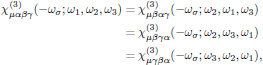
&+\underbrace{\chi^{(3)}_{\mu\alpha\beta\gamma}
(-\omega_{\sigma};\omega_1,\omega_2,\omega_3)
E_{\alpha}(\omega_1)E_{\beta}(\omega_2)E_{\gamma}(\omega_3)}_{
\sim P^{(3)}_{\mu}(\omega_{\sigma}),
\ \omega_{\sigma}=\omega_1+\omega_2+\omega_3}+\ldots\,]\cr
}
$$](/research/lectures/lect2/web/images_80proc/lect2_eq_disp_001.png) (1)
(1)where we adopted Einstein's convention of summation for terms with repeated subscripts. (A more formal formulation of the polarization density will be described later.)
2. Symmetries in nonlinear optics
There are essentially four classes of symmetries that we will encounter in this course:
-
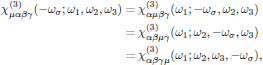
Intrinsic permutation symmetry:
that is to say, invariance under the n! possible permutations of (αk,ωk), k = 1, 2, … , n. This principle applies generally to resonant as well as nonresonant media. (Described in this lecture.)
-
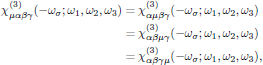
Overall permutation symmetry:
that is to say, invariance under the (n + 1)! possible permutations of (μ,-ωσ), (αk,ωk), k = 1, 2, … , n. This principle applies to nonresonant media, where all optical frequencies appearing in the formula for the susceptibility are removed far from the transition frequencies of the medium. (Described in detail in Lecture 4.)
-
Kleinman symmetry:
that is to say, invariance under the (n + 1)! possible permutations of μ, α1, …, αn. This principle is a consequence of the overall permutation symmetry, and applies in the low-frequency limit of nonresonant media.
- Spatial symmetries, given by the point symmetry class of the medium. (Described in detail in Lecture 6.)
3. Conditions for observing nonlinear optical interactions
Loosely formulated, a nonlinear response between light and matter depends on one of two key indgredients: either there is a resonance between the light wave and some natural oscillation mode of the medium, or the light is sufficiently intense. Direct resonance can occur in isolated intervals of the electromagnetic spectrum at
- ultraviolet and visible frequencies (∼ 1015 s-1) where the oscillator corresponds to an electronic transition of the medium,
- infrared (∼ 1013 s-1), where the medium has vibrational modes, and
- the far infrared-microwave range (∼ 1011 s-1) where there are rotational modes.
These interactions are also called one-photon processes, and are schematically illustrated in Fig. 3.
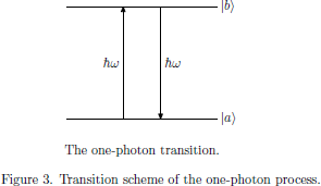
The lower frequency modes can be excited at optical frequencies (∼ 1015 s-1) through indirect resonant processes in which the difference in frequencies and wave vectors of two light waves, called the pump and Stokes wave, respectively, matches the frequency and wave vector of one of these lower frequency modes. These three-frequency interactions are sometime called two-photon processes. In the case where there "lower frequency" mode is an electronic transition or in the vibrational range (in which case the Stokes frequency can be of the same order of magnitude as that of the light wave), this process is called Raman scattering.
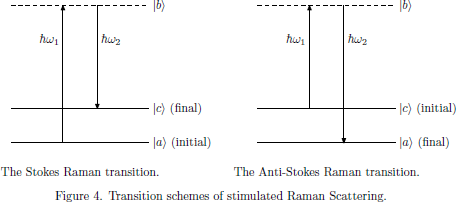
The stimulated Raman scattering is essentially a two-photon process in which one photon at ω1 is absorbed and one photon at ω2 is emitted, while the atom in the material undergoes a transition from the initial state |a> to the final state |c> Energy conservation requires the Raman resonance frequency (electronic or vibrational) to satisfy
 (2)
(2)and hence we may classify the Stokes and Anti-Stokes transitions as
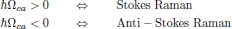 (3)
(3)When the lower frequency mode instead is an acoustic mode of the material, the process is instead called Brillouin scattering.
As will be shown explicitly later on in the course, optical resonance with transitions of the material is an important tool for "boosting up" the nonlinearities, with enhanced possibilities of applications. However, at single-photon resonance we have a strong absorption at the frequency of the optical field, and in most cases this is a non-desirable effect, since it decreases the optical intensity, even though it meanwhile also enhances the nonlinearity of the material.
However, by instead exploiting the two-photon resonance, the desired nonlinearity can be significantly enhanced whilst at the same time the competing absorption process can be minimized by avoiding coincidences between optical frequencies and single-photon resonances.
One general drawback with the resonant enhancement is that the response time of the polarization density of the material is slowed down, affecting applications such as optical switching or modulation, where speed is of importance.
4. Phenomenological description of the susceptibility tensors
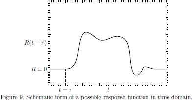
Before entering the full quantum-mechanical formalism, we will assume the medium to possess a temporal response described by time response functions R(t).
The very first step in the analysis is to express the electric polarization density, which in classical electrodynamical terms is expressed as the sum over all M electric charges qk at respective locations rk, all contained within a small volume V centered at r,
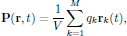 (4)
(4)as a series expansion
 (5)
(5)where P(1)(r,t) is linear in the electric field, P(2)(r,t) is quadratic in the electric field, and so on. The field-independent P(0)(r,t) corresponds to any possibly appearing static polarization of the medium. It should be emphasized that any of these terms may be linear as well as nonlinear functions of the electric field of the optical wave; that is to say, an externally applied static electric field may together with the electric field of the light interact through, for example, P(3)(r,t) to induce an electric polarization that is linear in the optical field.
In the analysis that now is to follow, we will a priori assume that it is possible to express the polarization density as a perturbation series. Later on, we will show how each of the terms can be derived from a more stringent basis, where it also will be stated which conditions that must hold in order to apply perturbation theory.
5. Linear polarization response function
Since P(1)(r,t) is taken as linear in the electric field, we may express the linear polarization density of the medium as being related to the optical field as
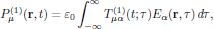 (6)
(6)
where
 is a rank-two tensor which weighs in all contributions in time from the
electric field of the light. A few required properties of this tensor can
immediately be stated:
is a rank-two tensor which weighs in all contributions in time from the
electric field of the light. A few required properties of this tensor can
immediately be stated:
-
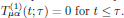
Causality. We require that no optically induced contribution can
occur before the field is applied, that is to say
- Time invariance. Under most circumstances, we may in addition assume that the material parameters are constant in time, such that P(1)(r,t') is identical to the polarisation as induced by the time-displaced electric field E(r,t').
The second of these properties is essentially a manifestation of an adiabatically following change of the carrier wave of the optical field.
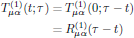
Using Eq. (6), the time invariance of the constitutive relation gives that
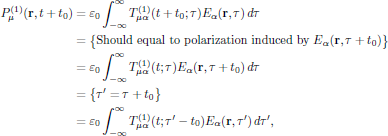 (7)
(7)from which we, by changing the dummy variable of integration back to τ, obtain the relation
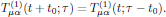
In particular, by setting t = 0 and replacing the arbitrary time displacement t0 by t, one finds that the response of the medium depends only of the time difference τ - t,
where we defined the linear polarization response function
 , being a rank-two tensor depending
only on the time difference τ - t.
, being a rank-two tensor depending
only on the time difference τ - t.
To summarize, the linear contribution to the electric polarization density is given in terms of the linear polarization response function as
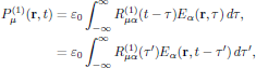 (8)
(8)and, and previously mentioned, the causality condition for the linear polarization response function requires that
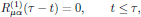 (9)
(9)and in addition, since the relation (8)is to hold for arbitrary time evolution of the electrical field, and since the polarization density P(1)μ(r,t) and the electric field Eα(r,t) both are real-valued quantities, we also require the polarization response function R(1)μα(τ-t) to be a real-valued function.
6. Quadratic polarization response function
The second-order, quadratic polarization density can in similar to the linear one be phenomenologically be written as the sum of all infinitesimal previous contributions in time. In this case, we must though include the possibility that not all contributions origin in the same time scale, and hence the proper formulation of the second order polarization density is as a two-dimensional integral,
 (10)
(10)
The tensor
 uniquely
determines the quadratic, second-order polarization of the medium.
However, this tensor is not per se unique. To see this, we may
express the tensor as a sum of a symmetric part and an antisymmetric part,
uniquely
determines the quadratic, second-order polarization of the medium.
However, this tensor is not per se unique. To see this, we may
express the tensor as a sum of a symmetric part and an antisymmetric part,
![$$
\eqalign{
T^{(2)}_{\mu\alpha\beta}(t;\tau_1,\tau_2)
&={{1}\over{2}}
\underbrace{
\bigg[T^{(2)}_{\mu\alpha\beta}(t;\tau_1,\tau_2)
+T^{(2)}_{\mu\beta\alpha}(t;\tau_2,\tau_1)\bigg]
}_{\rm symmetric}
+{{1}\over{2}}
\underbrace{
\bigg[T^{(2)}_{\mu\alpha\beta}(t;\tau_1,\tau_2)
-T^{(2)}_{\mu\beta\alpha}(t;\tau_2,\tau_1)\bigg]
}_{\rm antisymmetric}\cr
&=\underbrace{S^{(2)}_{\mu\alpha\beta}(t;\tau_1,\tau_2)}_{
=S^{(2)}_{\mu\beta\alpha}(t;\tau_2,\tau_1)}
+\underbrace{A^{(2)}_{\mu\alpha\beta}(t;\tau_1,\tau_2)}_{
=-A^{(2)}_{\mu\beta\alpha}(t;\tau_2,\tau_1)}\cr
}
$$](/research/lectures/lect2/web/images_80proc/lect2_eq_disp_017.png) (11)
(11)As this form of the response function is inserted into the original expression (10) for the second order polarization density, we immediately find that it is left invariant under the interchange of the dummy variables (α,τ1) and (β,τ2) (since the integration is performed from minus to plus infinity in time). In particular, it from this follows that
![$$
\eqalign{
P^{(2)}_{\mu}({\bf r},t)&=\varepsilon_0
\int^{\infty}_{-\infty}\int^{\infty}_{-\infty}
[S^{(2)}_{\mu\alpha\beta}(t;\tau_1,\tau_2)
+A^{(2)}_{\mu\alpha\beta}(t;\tau_1,\tau_2)]
E_{\alpha}({\bf r},\tau_1) E_{\beta}({\bf r},\tau_2)
\,d\tau_1\,d\tau_2\cr
&=\varepsilon_0
\underbrace{\int^{\infty}_{-\infty}\int^{\infty}_{-\infty}
S^{(2)}_{\mu\alpha\beta}(t;\tau_1,\tau_2)
E_{\alpha}({\bf r},\tau_1) E_{\beta}({\bf r},\tau_2)
\,d\tau_1\,d\tau_2}_{\equiv I_1}\cr&\qquad
+\varepsilon_0
\underbrace{\int^{\infty}_{-\infty}\int^{\infty}_{-\infty}
A^{(2)}_{\mu\alpha\beta}(t;\tau_1,\tau_2)
E_{\alpha}({\bf r},\tau_1) E_{\beta}({\bf r},\tau_2)
\,d\tau_1\,d\tau_2}_{\equiv I_2}\cr
&=\varepsilon_0
\int^{\infty}_{-\infty}\int^{\infty}_{-\infty}
S^{(2)}_{\mu\beta\alpha}(t;\tau_2,\tau_1)
E_{\alpha}({\bf r},\tau_1) E_{\beta}({\bf r},\tau_2)
\,d\tau_1\,d\tau_2\cr&\qquad
-\varepsilon_0
\int^{\infty}_{-\infty}\int^{\infty}_{-\infty}
A^{(2)}_{\mu\beta\alpha}(t;\tau_2,\tau_1)
E_{\alpha}({\bf r},\tau_1) E_{\beta}({\bf r},\tau_2)
\,d\tau_1\,d\tau_2\cr
&=\varepsilon_0
\underbrace{\int^{\infty}_{-\infty}\int^{\infty}_{-\infty}
S^{(2)}_{\mu\beta\alpha}(t;\tau_2,\tau_1)
E_{\beta}({\bf r},\tau_2) E_{\alpha}({\bf r},\tau_1)
\,d\tau_1\,d\tau_2}_{=I_1}\cr&\qquad
-\varepsilon_0
\underbrace{\int^{\infty}_{-\infty}\int^{\infty}_{-\infty}
A^{(2)}_{\mu\beta\alpha}(t;\tau_2,\tau_1)
E_{\beta}({\bf r},\tau_2) E_{\alpha}({\bf r},\tau_1)
\,d\tau_1\,d\tau_2}_{=I_2}\cr
}
$$](/research/lectures/lect2/web/images_80proc/lect2_eq_disp_018.png)
that is to say, the symmetric part satisfies the trivial identity I1 = I1, while the antisymmetric part satisfies I2 = -I2, which shows that the antisymmetric part does not contribute to the polarization density, and that we may set the antiymmetric part to zero, without imposing any constraint on the validity of the theory.
The time response T(2)μαβ(t;τ1,τ2) is then unique and is from now on chosen to be symmetric,
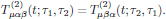 (12)
(12)This procedure of symmetrization may seem like an all-theoretical contruction, somewhat out of focus of what lies ahead, but in fact it turns out to be an extremely useful property that we later on will exploit extensively. The previously described symmetric property will later on, for susceptibility tensors in the frequency domain, be denoted as the intrinsic permutation symmetry, a general property that will hold irregardless of whether the nonlinear interaction under analysis is highly resonant or far from resonance.
By again applying the arguments of time invariance, as previously for the linear response function, we find that

for all t, τ1, and τ2. Hence, by setting t = 0 and then replacing the arbitrary time t0 by t, again as previously done for the linear case, one finds that T(2)(t;τ1,τ2) depends only on the two time differences t - τ1 and t - τ2. To make this fact explicit, we may hence write the response function as
 (13)
(13)giving the canonical form of the quadratic polarization density as
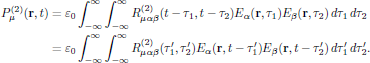 (14)
(14)
The tensor
 is denoted the
quadratic electric polarization response of the medium,
and in similar with the linear response function, arguments
of causality require the response function to be zero whenever
τ1 and/or τ2 is negative. Similarly, the reality
condition on Eα(r,t) and
Pα(r,t)
requires that the quadratic electric polarization response of the medium
is a real-valued function.
is denoted the
quadratic electric polarization response of the medium,
and in similar with the linear response function, arguments
of causality require the response function to be zero whenever
τ1 and/or τ2 is negative. Similarly, the reality
condition on Eα(r,t) and
Pα(r,t)
requires that the quadratic electric polarization response of the medium
is a real-valued function.
7. Higher order polarization response functions
The n:th order polarization density can in similar to the linear (n = 1) and quadratic (n = 2) ones be written as
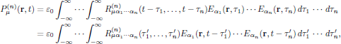
where the n:th order response function is a tensor of rank n + 1, and a real-valued function of the n parameters τ1, … , τn, vanishing whenever any τk < 0, k = 0, 1, … , n, and with the intrinsic permutation symmetry that it is left invariant under any of the n! pairwise permutations of (α1,τ1), … , (αn,τn).