Lectures on Nonlinear Optics - Lecture 1
Introduction to Nonlinear Optics
lect1.pdf [283 kB] Lecture 1 in Portable Document Format.
Nonlinear optics is the discipline in physics in which the electric polarization density of the medium is studied as a nonlinear function of the electromagnetic field of the light. Being a wide field of research in electromagnetic wave propagation, nonlinear interaction between light and matter leads to a wide spectrum of phenomena, such as optical frequency conversion, optical solitons, phase conjugation, and Raman scattering. In addition, many of the analytical tools applied in nonlinear optics are of general character, such as the perturbative techniques and symmetry considerations, and can equally well be applied in other disciplines in nonlinear dynamics.
Contents
- The contents of the course
- Examples of applications of nonlinear optics
- A brief history of nonlinear optics
- Outline for calculations of polarization densities
- Introduction to nonlinear dynamical systems
- The anharmonic oscillator
1. The contents of this course
This course is intended as an introduction to the wide field of phenomena encountered in nonlinear optics. The course covers:
- The theoretical foundation of nonlinear interaction between light and matter.
- Perturbation analysis of nonlinear interaction between light and matter.
- The Bloch equation and its interpretation.
- Basics of soliton theory and the inverse scattering transform.
It should be emphasized that the course does not cover state-of-the-art material constants of nonlinear optical material etc., but rather focus on the theoretical foundations and ideas of nonlinear optical interactions between light and matter.
A central analytical technique in this course is the perurbation analysis, with its foundation in the analytical mechanics. This technique will in the course mainly be applied to the quantum-mechanical description of interaction between light and matter, but is central in a wide field of cross-disciplinary physics as well. In order to give an introduction to the analytical theory of nonlinear systems, we will therefore start with the analysis of the nonlinear equations of motion for the mechanical pendulum.
2. Examples of applications of nonlinear optics
Some important applications in nonlinear optics:
- Optical parametric amplification (OPA) and oscillation (OPO), ωp → ωs + ωi. (Light at pump angluar frequency ωp generates a signal wave at ωs and an idler at ωi)
- Second harmonic generation (SHG), ω + ω → 2ω. (Light at pump angluar frequency ω generates a second-harmonic wave at 2ω, or half the vacuum wavelength)
- Third harmonic generation (THG), ω + ω + ω → 3ω.
- Pockels effect, or the linear electro-optical effect (applications for optical switching).
- Optical bistability (optical logics).
- Optical solitons (ultra long-haul communication).
3. A brief history of nonlinear optics
Some important advances in nonlinear optics:
- Townes et al. (1960), invention of the laser. Charles H. Townes was in 1964 awarded the Nobel Prize for the invention of the ammonia laser. His Nobel Lecture can be found here.
- Franken et al. (1961), First observation ever of nonlinear optical effects, second harmonic generation (SHG). (Franken et al. detected ulvtraviolet light (λ=347.1 nm) at twice the frequency of a ruby laser beam (λ=694.2 nm) when this beam traversed a quartz crystal; P. A. Franken, A. E. Hill, C. W. Peters, G. Weinreich, Phys. Rev. Lett. 7, 118 (1961).) Second harmonic generation is also the first nonlinear effect ever observed where a coherent input generates a coherent output.
- Terhune et al. (1962), First observation of third harmonic generation (THG). (Noteworthy is that in their seminal experiment, Terhune et al. detected only about a thousand THG photons per pulse, at λ=231.3 nm, corresponding to a conversion of one photon out of about 1015 photons at the fundamental wavelength at λ=693.9 nm; see R. W. Terhune, P. D. Maker, and C. M. Savage, Phys. Rev. Lett. 8, 404 (1962).
- E. J. Woodbury and W. K. Ng (1962), first demonstration of stimulated Raman scattering. E. J. Woodbury and W. K. Ng, Proc. IRE {\bf 50}, 2347 (1962).
- Armstrong et al. (1962), formulation of the general permutation symmetry relations in nonlinear optics. (The general permutation symmetry relations of higher-order susceptibilities were published by J. A. Armstrong, N. Bloembergen, J. Ducuing, and P. S. Pershan, Phys. Rev. 127, 1918 (1962).) This seminal article formulates one of the theoretical corner stones upon which this course relies, and will be discussed in extent later on.
- A. Hasegawa and F. Tappert (1973), the first theoretical prediction of soliton generation in optical fibers. A. Hasegawa and F. Tappert, Transmission of stationary nonliner optica pulses in dispersive optical fibers: I, Anomalous dispersion; II Normal dispersion, Appl. Phys. Lett. 23, 142-144 and Appl. Phys. Lett. 23, 171-172 (August 1 and 15, 1973), respectively.
- H. M. Gibbs et al. (1976), first demonstration and explaination of optical bistability. H. M. Gibbs, S. M. McCall, and T. N. C. Venkatesan, Phys. Rev. Lett. 36, 1135 (1976).
- L. F. Mollenauer et al. (1980), first confirmation of soliton generation in optical fibers. [L. F. Mollenauer, R. H. Stolen, and J. P. Gordon, Experimental observation of picosecond pulse narrowing and solitons in optical fibers, Phys. Rev. Lett. 45, 1095-1098 (September 29, 1980)]; the first reported observation of solitons was though made in 1834 by John Scott Russell, a Scottish scientist and later famous Victorian engineer and shipbuilder, while studying water waves in the Glasgow-Edinburgh channel.
Recently, many advances in nonlinear optics has been made, with a lot of efforts with fields of, for example, Bose-Einstein condensation and laser cooling; these fields are, however, a bit out of focus from the subjects of this course, which can be said to be an introduction to the 1960s and 1970s advances in nonlinear optics. It should also be emphasized that many of the effects observed in nonlinear optics, such as the Raman scattering, were observed much earlier in the microwave range.
4. Outline for calculations of polarization densities
4.1 Metals and plasmas
From an all-classical point-of-view, the calculation of the electric polarization density of metals and plasmas, containing a free electron gas, can be performed using the model of free charges acting under the Lorenz force of an electromagnetic field,
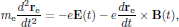 (1)
(1)where E(t) and B(t) are all-classical electric and magnetic fields of the electromagnetic field of the light. In forming the equation (1) for the motion of the electron, the origin was chosen to coincide with the center of the nucleus.
4.2 Dielectrics
A very useful model used by Drude and Lorentz [R. Becker, Elektronen Theorie, (Teubner, Leipzig, 1933), in German] to calculate the linear electric polarization of the medium describes the electrons as harmonically bound particles.
For dielectrics in the nonlinear optical regime, as being the focus of our attention in this course, the calculation of the electric polarization density is instead performed using a nonlinear spring model of the bound charges, here quoted for one-dimensional motion as
 (2)
(2)As in the previous case of metals and plasmas, in forming the equation for the motion of the electron, the origin was also here chosen to coincide with the center of the nucleus.
The classical mechanical model expressed by Eq. (2) will later in this lecture be applied to the derivation of the second-order nonlinear polarzation density of the medium.
5. Introduction to nonlinear dynamical systems
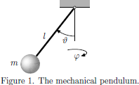
In this section we will, as a preamble to later analysis of quantum-mechanical systems, apply perturbation analysis to a simple mechanical system. Among the simplest nonlinear dynamical systems is the pendulum, for which the total mechanical energy of the system, considering the point of suspension as defining the level of zero potential energy, is given as the sum of the kinetic and potential energy as
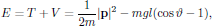 (3)
(3)where m is the mass, g the gravitation constant, l the length, and ϑ the angle of deflection of the pendulum, and where p is the momentum of the point mass.
From the total mechanical energy of the system, as provided by Eq. (3), the equations of motion for the point mass is hence given by Lagranges equations (see Goldstein's Classical Mechanics [5]),
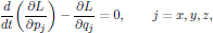 (4)
(4)where qj are the generalized coordinates,
 (5)
(5)are the components of the generalized momentum, and
 (6)
(6)is the Lagrangian of the mechanical system. In spherical coordinates (ρ,φ,ϑ), the momentum for the point mass is given as its mass times the velocity,
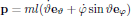 (7)
(7)and the Lagrangian for the pendulum is hence given as
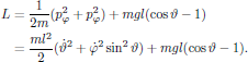 (8)
(8)As the Lagrangian (8) for the pendulum is inserted into Eq. (4), the resulting equations of motion are for qj = φ and ϑ obtained as
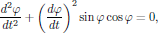 (9)
(9)and
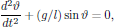 (10)
(10)respectively, where we observe that the motion in the eφ and eϑ directions are decoupled. We may also notice that the equation of motion for φ is independent of any of the physical parameters involved in the Lagrangian, and the evolution of φ(t) in time is entirely determined by the initial conditions at some time t = t0.
In the following discussion, the focus will be on the properties of the motion of ϑ(t). The equation of motion (10) for the ϑ coordinate is here described by the so-called Sine-Gordon equation [1]. This nonlinear differential equation is hard [2] to solve analytically, but if the nonlinear term is expanded as a Taylor series around ϑ = 0,
 (11)
(11)we may proceed with an approximate solution, even inclusing the first-order nonlinearity which appear in the equation.
Before proceeding further with the properties of the solutions to the approximative Sine-Gordon equation (11), including various orders of nonlinearities, the general technique of solving the equation by means of perturbation analysis will now be illustrated. In order to illustrate the behaviour of the Sine-Gordon equation, we may, for the sake of simplicity in the expressions, normalize it by using the normalized time τ = (g/l)1/2t, giving the Sine-Gordon equation in the standard normalized form
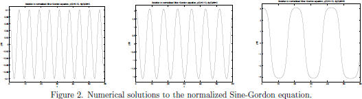
 (12)
(12)The numerical solutions to the normalized Sine-Gordon equation are in Fig. 2 shown for initial conditions (a) y(0) = 0.1, (b) y(0)=2.1, and (c) y(0)=3.1, all cases with y'(0)=0.
First of all, we may consider the linear case, for which the approximation sinϑ ≈ ϑ holds. For this case, the Sine-Gordon equation (12) reduces to the one-dimensional linear wave-equation, with the standard solution
 (13)
(13)As seen in the frequency domain, this solution gives a delta peak at ω = (g/l)1/2 in the power spectrum |ϑ(ω)|2, with no other frequency components present (as we expect). However, if we include the nonlinearities, the previous sine-wave solution will tend to flatten at the peaks, as well as increase in period, and this changes the power spectrum to be broadened as well as flattened out. In other words, the solution to the Sine-Gordon give rise to a wide spectrum of frequencies, as compared to the delta peaks of the solutions to the linearized, approximative Sine-Gordon equation.
From the numerical solutions, we may draw the conclusion that whenever higher order nonlinear restoring forces come into play, even such a simple mechanical system as the pendulum will carry frequency components at a set of frequencies differing from the single frequency given by the linearized model of motion.
More generally, for a moment hiding the fact that for this particular case the restoring force is a simple sine function, the equation of motion for the pendulum can be written as
 (14)
(14)This equation of motion may be compared with the nonlinear wave equation for the electromagnetic field of a travelling optical wave of angular frequency $\omega$, of the form
 (15)
(15)which clearly shows the similarity between the nonlinear wave propagation and the motion of the nonlinear pendulum.
Having solved the particular problem of the nonlinear pendulum, we may ask ourselves if the equations of motion may be altered in some way in order to give insight in other areas of nonlinear physics as well. For example, the series (14), which defines the feedback that tend to restore the mechanical pendulum to its rest position, clearly defines equations of motion that conserve the total energy of the mechanical system. This, however, in generally not true for an arbitrary series of terms of various power for the restoring force. As we will later on see, in nonlinear optics we generally have a complex, though in many cases most predictable, transfer of energy between modes of different frequencies and directions of propagation.
6. The anharmonic oscillator
Among the simplest models of interaction between light and matter is the all-classical one-electron oscillator, consisting of a negatively charged particle (electron) with mass me, mutually interacting with a positively charged particle (proton) with mass mp, through attractive Coulomb forces.
In the one-electron oscillator model, several levels of approximations may be applied to the problem, with increasing algebraic complexity. At the first level of approximation, the proton is assumed to be fixed in space, with the electron free to oscillate around the proton. Quite generally, at least within the scope of linear optics, the restoring spring force which confines the electron can be assumed to be linear with the displacement distance of the electron from the central position. Providing the very basic models of the concept of refractive index and optical dispersion, this model has been applied by numerous authors, such as Feynman [3], and Born and Wolf [4].
Moving on to the next level of approximation, the bound proton-electron pair may be considered as constituting a two-body central force problem of classical mechanics, in which one may assume a fixed center of mass of the system, around which the proton as well as the electron are free to oscillate. In this level of approximation, by introducing the concept of reduced mass for the two moving particles, the equations of motion for the two particles can be reduced to one equation of motion, for the evolution of the electric dipole moment of the system.
The third level of approximation which may be identified is when the center of mass is allowed to oscillate as well, in which case an equation of motion for the center of mass appears in addition to the one for the evolution of the electric dipole moment.
In each of the models, nonlinearities of the restoring central force field may be introduced as to include nonlinear interactions as well. It should be emphasized that the spring model, as now will be introduced, gives an identical form of the set of nonzero elements of the susceptibility tensors, as compared with those obtained using a quantum mechanical analysis.
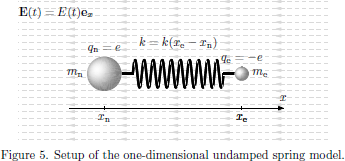
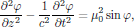
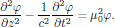
Throughout this analysis, the wavelength of the electromagnetic field will be assumed to be sufficiently large in order to neglect any spatial variations of the fields over the spatial extent of the oscillator system. In this model, the central force field is modelled by a mechanical spring force with spring constant ke, as shown schematically in Fig. 5, and the all-classical Newton's equations of motion for the electron and nucleus are
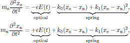
corresponding to a system of two particles connected by a spring with spring "constant"
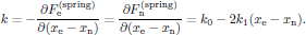 (17)
(17)By introducing the reduced mass [5]
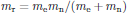 (18)
(18)of the system, the equation of motion for the electric dipole moment
 (19)
(19)then becomes
 (20)
(20)This inhomogeneous nonlinear ordinary differential equation for the electric dipole moment is the primary interest in the discussion that now is to follow.
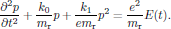
The electric dipole moment of the anharmonic oscillator is now expressed in terms of a perturbation series as
 (21)
(21)where each term in the series is proportional to the applied electrical field strength to the power as indicated in the superscript of repective term, and formulate the system of n + 1 equations for p(k), k = 0, 1, 2, ... , n, that define the time evolution of the electric dipole. By inserting the perturbation series of Eq. (21)into Eq. (20), we hence obtain the equation of motion for the dipole moment as
 (22)
(22)Since this equation is to hold for an arbitrary electric field E(t), that is to say, at least within the limits of the validity of the perturbation analysis, each set of terms with equal power dependence of the electric field must individually satisfy the relation. By sorting out the various powers and identifying terms in the left and right hand sides of Eq. (22), we arrive at the system of equations
 (23)
(23)where we kept terms with powers of the electric field up to and including order three. At a first glance, this system seem to suggest that only the first order of the perturbation series depends on the applied electric field of the light; however, taking a closer look at the system, one can easily verify that all orders of the dipole moment is coupled directly to the lower order terms. The system of equations for p(k) can now be solved for k = 0, 1, 2, ... , n (in this very order), to successively provide the basis of solutions for higher and higher order terms, until reaching some k = n after which we safely may neglect the reamaining terms, hence providing an approximate solution. It should though be emphasized that in the limit n → ∞, the described theory still is an exact description of the motion of the electric dipole moment within this model of interaction between light and matter.
The zeroth order term in the perturbation series is decribed by a nonlinear ordinary differential equation of order two, a so-called Riccati equation, which analytically can be solved exactly, either by directly applying the theory of Jacobian elliptic integrals of by applying the Riccati transormation. (For examples of the application of the Riccati transformation, see Zwillinger [6].) However, by considering a system starting from rest, at a state of equilibrium, we can immediately draw the conclusion that p(0)(t) must be identically zero for all times t. This, of course, only holds for this particular model; in many molecular systems, such in water, a permanent static dipole moment is present, something that is left out in this particular spring model of ours. (Not to be confused with the static polarization induced by the electric field, which by definition of the terms in the perturbation series is included in higher order terms, depending on the power of the electric field.)
The first order term in the perturbation series is the first and only one with an explicit dependence of the electric field of the light. Since the zeroth order perturbation term is zero, the differential equation for the first order term is linear, which simplifies the calculus. However, since it is an inhomogeneous differential equation, we must generally look for a total solution to the equation as a sum of a homogeneous solution (with zero right hand side) and a particular solution (with the electric field in the right hand side present). The homogeneous solution, which will contain two constants of integration (since we are considering second-order ordinary differential equation) will though only give the part of the solution which depend on initial conditions, that is to say, in this case a harmonic natural oscillation of the spring system which in the presence of damping terms rapidly would decrease to zero. This implies that in order to find steady-state solutions, in which the oscillation of the dipole moment directly follows the oscillation of the electric field of the light, we may directly start looking for the particular solution. For a time harmonic electric field, here taken as
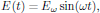 (24)
(24)the particular solution for the first order term is after some straightforward algebra given as [7]
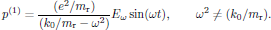 (25)
(25)For a material consisting of N dipoles per unit volume, and by following the conventions for the linear electric susceptibility in SI units, this corresponds to a first order electric polarization density of the form
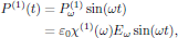 (26)
(26)with the first order (linear) electric susceptibility given as
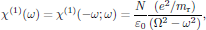 (27)
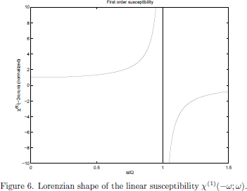
(27)where the resonance frequency Ω2 = k0/mr was introduced. The Lorenzian shape of the frequency dependence is shown in Fig. 6.
Continuing with the second order perturbation term, some straightforward algebra gives that the particular solution for the second order term of the electric dipole moment becomes
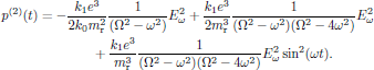 (28)
(28)In terms of the polarization density of the medium, still with N dipoles per unit volume and following the conventions in regular SI units, this can be written as
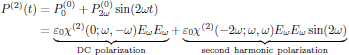 (29)
(29)with the second order (quadratic) electric susceptibility given as
![$$
\eqalign{
\chi^{(2)}(0;\omega,-\omega)&=
{{N}\over{\varepsilon_0}}{{k_1e^3}\over{2m^3_{\rm r}}}
\bigg[{{1}\over{(\Omega^2-\omega^2)(\Omega^2-4\omega^2)}}
-{{1}\over{\Omega^2(\Omega^2-\omega^2)}}\bigg],\cr
\chi^{(2)}(2\omega;\omega,\omega)&=
{{N}\over{\varepsilon_0}}{{k_1e^3}\over{m^3_{\rm r}}}
{{1}\over{(\Omega^2-\omega^2)(\Omega^2-4\omega^2)}}.\cr
}
$$](/research/lectures/lect1/web/images_80proc/lect1_eq_disp_029.png) (30)
(30)From this we may notice that for one-photon resonances, the nonlinearities are enhanced whenever ω → Ω or 2ω → Ω for the induced DC as well as the second harmonic polarization density.
The explicit frequency dependencies of the susceptibilities χ(2)(-2ω;ω,ω) and χ(2)(0;ω,-ω) are shown in Figs. 7 and 8.
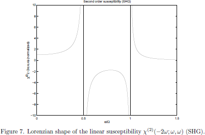
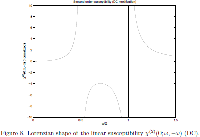
A well known fact in electromagnetic theory is that an electric dipole that oscillates at a certain angular frequency, say at $2\omega$, also emits electromagnetic radiation at this frequency. In particular, this implies that the term described by the susceptibility χ(2)(-2ω;ω,ω) will generate light at twice the angular frequency of the light, hence generating a second harmonic light wave.
References
[1] The term "Sine-Gordon equation" has its origin as an allegory over the similarity between the time-dependent (Sine-Gordon) equation
appearing in, for example, relativistic field theories, as compared to the time-dependent Klein-Gordon equation, which takes the form
The Sine-Gordon equation is sometimes also called "pendulum equation" in the terminology of classical mechanics.
[2] Impossible?
[3] R. P. Feynman, Lectures on Physics (Addison-Wesley, Massachusetts, 1963).
[4] M. Born and E. Wolf, Principles of Optics (Cambridge University Press, Cambridge, 1980).
[5] Herbert Goldstein, Classical Mechanics, 2nd Ed. (Addison-Wesley, Massachusetts, 1980).
[6] Daniel I. Zwillinger, Handbook of Differential Equations, 2nd Ed. (Academic Press, Boston, 1992).
[7] For the sake of self-consistency, the general solution for the first order term is given as

where A and B are constants of integration, determined by initial conditions.